Introduction to Python for Data Science

Getting Started: Your Python and Jupyter Environment¶

Welcome to the world of Python for data science! This notebook will guide you through the basics of Python and its essential tools, setting you up for more advanced data analysis techniques.

To effectively run the labs and exercises in this book, you will need the following:

• Python 3 Installation: We’ll be using Python 3, the current and widely supported version of the language. Python is the workhorse behind many data science tasks, known for its readability and extensive libraries.
• Jupyter Notebook Access: Jupyter is an interactive environment that allows you to write and run code, visualize results, and document your process all in one place. It’s a fantastic tool for learning and exploring data.

Installing Python and Anaconda:

The easiest way to get both Python 3 and Jupyter, along with many useful data science packages, is by installing Anaconda. Anaconda is a free and open-source distribution of Python and R, specifically designed for scientific computing and data science.

1. Download Anaconda: Go to anaconda.com and download the Python 3 version appropriate for your operating system (Windows, macOS, or Linux).
2. Installation: Follow the on-screen instructions to install Anaconda on your system. Anaconda will install Python, Jupyter, and a host of popular packages like NumPy, Pandas, and Matplotlib, which we’ll be using extensively.

Accessing Jupyter Notebook:

Once Anaconda is installed, you have several options to access Jupyter:

• Google Colaboratory (Colab): colab.research.google.com/ - Colab is a free cloud-based Jupyter Notebook environment provided by Google. It requires no installation and is a great way to get started quickly. Simply open your browser, go to the link, and you can begin coding.
• JupyterHub: jupyter.org/hub - JupyterHub provides a multi-user Jupyter environment that can be accessed through a web browser. This is often used in educational or organizational settings.
• Local Jupyter Installation: If you installed Anaconda, you already have Jupyter installed locally on your computer. You can launch it in a few ways:
  • Anaconda Navigator: Open Anaconda Navigator (installed with Anaconda) and launch JupyterLab or Jupyter Notebook from there.
  • Command Line/Terminal: Open your command prompt (Windows) or terminal (macOS/Linux) and type jupyter lab or jupyter notebook and press Enter. This will open Jupyter in your web browser.

For detailed, up-to-date instructions on setting up Python and Jupyter, please refer to the “Python resources” page on the book website statlearning.com.

Installing the ISLP Package:

The ISLP package is specifically designed to accompany this book. It provides convenient access to datasets and custom functions that we will use throughout the labs. It also conveniently installs many other packages that are commonly used in data science.

To install ISLP, open your terminal or Anaconda Prompt and type the following command:

Press Enter to execute the command. pip is the package installer for Python. This command will download and install the ISLP package and its dependencies.

For more information about the ISLP package, including documentation and available datasets, visit the ISLP documentation website linked from the “Python resources” page.

Running this Lab Notebook:

1. Download the Notebook: Download the file Ch2-statlearn-lab.ipynb from the “Python resources” page on the book website. This file contains the code and exercises for this lab.
2. Navigate to the Notebook Directory: In your terminal or command prompt, navigate to the directory where you downloaded Ch2-statlearn-lab.ipynb. You can use the cd command (change directory) for this. For example, if you downloaded it to your “Downloads” folder, you might type cd Downloads.
3. Launch Jupyter Lab: In the same terminal or command prompt, type jupyter lab Ch2-statlearn-lab.ipynb and press Enter. This command will open Jupyter Lab in your web browser, and the Ch2-statlearn-lab.ipynb notebook should be open and ready to use.

Windows Users:

If you are using Windows, you can access Anaconda and its tools through the Start Menu. Look for “Anaconda Prompt” or “Anaconda Powershell Prompt” in your Start Menu. Opening one of these will give you a command-line interface where you can run the pip install ISLP and jupyter lab Ch2-statlearn-lab.ipynb commands as described above.

Let’s begin our Python journey!

Basic Commands: Interacting with Python¶

Let’s start with the fundamental building blocks of Python. Like any programming language, Python uses functions to perform actions. Functions are reusable blocks of code designed to carry out specific tasks.

To use a function, you “call” it by typing its name followed by parentheses (). Inside the parentheses, you can provide inputs or arguments that tell the function how to operate. A function can take zero, one, or multiple inputs.

One of the most basic functions is print(). The print() function displays the output of whatever you provide as its arguments to the console (or in the output cell of a Jupyter notebook).

In the code above, "fit a model with", 11, and "variables" are the arguments passed to the print() function. print() takes these arguments and displays them as text.

Getting Help with Functions:

Python provides a built-in way to get help and documentation about functions. To see the documentation for any function, you can type the function name followed by a question mark ? and run the cell.

Running this will display the documentation for the print() function, explaining its purpose, arguments, and usage. This is an invaluable tool for learning about new functions and understanding how to use them correctly.

Basic Arithmetic:

Python can perform mathematical calculations just like a calculator. Adding numbers is straightforward:

Python understands standard arithmetic operators like + (addition), - (subtraction), * (multiplication), / (division), and ** (exponentiation).

Strings: Working with Text:

In Python, text is represented using strings. Strings are sequences of characters and are enclosed in either single quotes ' ' or double quotes " ".

Here, we are using the + operator to concatenate (join together) strings. Python treats strings as sequences, and the + operator, when used with strings, performs concatenation rather than addition.

Lists: Ordered Collections of Items:

Python lists are versatile data structures that hold ordered collections of items. Lists are defined using square brackets [] and items within a list are separated by commas ,. Lists can contain items of different data types (numbers, strings, even other lists!).

In this example, we’ve created a list named x containing the numbers 3, 4, and 5. When you type the name of a variable in Jupyter and run the cell, Python displays the value of that variable, which in this case is the list [3, 4, 5].

List Concatenation vs. Element-wise Operations:

Let’s explore what happens when we try to “add” two lists:

The result might be surprising if you were expecting element-wise addition (like adding the first element of x to the first element of y, the second to the second, and so on). Instead, Python concatenates the lists, meaning it joins them end-to-end. This is because, in Python, lists are designed to hold arbitrary objects, not just numbers for mathematical operations.

This behavior highlights a crucial point: Python is a general-purpose programming language. While it’s powerful for data science, many data-specific functionalities come from external packages or libraries. For numerical computations and data manipulation, we’ll rely heavily on packages like numpy and pandas.

In the next section, we’ll dive into numpy, which provides efficient tools for numerical operations, especially with arrays and matrices. For more comprehensive information about basic Python concepts, you can explore the official Python tutorial: docs.python.org/3/tutorial/.

Introduction to Numerical Python (NumPy)¶

As we’ve seen, standard Python lists are not optimized for numerical operations like element-wise addition or matrix manipulations. This is where NumPy (Numerical Python) comes to the rescue. NumPy is a fundamental library in Python for scientific computing. It provides powerful tools for working with arrays, matrices, and performing efficient numerical computations.

NumPy introduces a new data structure called the NumPy array, which is designed for numerical data and operations. NumPy arrays are more efficient and versatile than standard Python lists for numerical tasks.

To use NumPy, we first need to import it into our Python environment. It’s convention to import NumPy using the abbreviation np for easier access to its functions.

This line imports the NumPy library and gives it the alias np. Now, whenever we want to use a NumPy function or object, we’ll prefix it with np..

Creating NumPy Arrays:

We can create NumPy arrays from Python lists using the np.array() function.

Here, we’ve created two NumPy arrays, x and y, from the lists we defined earlier. Notice the syntax np.array(). This indicates that we are calling the array() function from the numpy package (which we’ve aliased as np).

Element-wise Operations with NumPy Arrays:

Now, let’s try adding our NumPy arrays x and y:

This time, the result is what we intuitively expected: element-wise addition! NumPy arrays are designed for numerical computations, and arithmetic operations like +, -, *, / are performed element-wise when applied to NumPy arrays.

Multidimensional Arrays (Matrices):

NumPy arrays can be multidimensional, making them ideal for representing matrices and tensors. A two-dimensional NumPy array is essentially a matrix.

This creates a 2x2 matrix (a two-dimensional array) represented by x. The outer square brackets [] enclose the rows, and the inner square brackets enclose the elements within each row.

Array Attributes:

NumPy arrays have various attributes that provide information about the array itself. You can access an attribute using dot notation: array_name.attribute_name.

For example, ndim attribute tells you the number of dimensions of the array:

The output 2 indicates that x is a two-dimensional array (a matrix).

The dtype attribute tells you the data type of the elements in the array.

The output int64 (or similar, depending on your system) indicates that the elements of x are 64-bit integers. NumPy arrays store elements of the same data type, which contributes to their efficiency.

Data Type Conversion:

NumPy automatically infers the data type based on the input data. If you provide integers, it creates an integer array. If you include a decimal number, it will create a floating-point array.

Here, even though most elements are integers, the presence of 3.0 (a float) forces NumPy to create a floating-point array (float64).

You can also explicitly specify the desired data type when creating an array using the dtype argument:

This explicitly creates a floating-point array, even though the input values are integers.

Array Shape:

The shape attribute of a NumPy array returns a tuple (an immutable sequence) indicating the dimensions of the array. For a matrix, the shape is (rows, columns).

For our 2x2 matrix x, the output (2, 2) confirms it has 2 rows and 2 columns.

Array Methods and NumPy Functions:

NumPy arrays have methods, which are functions associated with the array object itself. You call a method using dot notation: array_name.method_name().

For example, the sum() method calculates the sum of all elements in the array.

Alternatively, NumPy also provides stand-alone functions that operate on arrays. For example, np.sum() function also calculates the sum of array elements.

In many cases, both methods and functions achieve the same result. Choosing between them often comes down to personal preference or code readability.

Reshaping Arrays:

The reshape() method allows you to change the shape of an array without altering its data. It returns a new array with the specified shape.

Here, we reshaped the 1D array x into a 2D array x_reshape with 2 rows and 3 columns. NumPy fills the reshaped array in row-major order, meaning it fills row by row.

Indexing NumPy Arrays:

NumPy uses zero-based indexing, meaning the first element of an array is at index 0, the second at index 1, and so on. For multidimensional arrays, you index using comma-separated indices within square brackets [].

This accesses the element at the first row (index 0) and first column (index 0) of x_reshape.

This accesses the element at the second row (index 1) and third column (index 2).

Similarly, for a one-dimensional array:

This accesses the third element (index 2) of x.

Views vs. Copies in NumPy:

A crucial concept in NumPy is the distinction between views and copies. In some cases, operations on arrays create views, which are just different ways of looking at the same underlying data. Changes to a view will affect the original array. In other cases, operations create copies, which are independent arrays with their own data.

Let’s see an example of a view:

Notice that modifying x_reshape also changed the original array x! This is because x_reshape (in this case) is a view of x. Reshaping, in many situations, creates a view rather than a copy to save memory and improve performance.

Tuples vs. Lists (Briefly):

We encountered tuples when discussing array shapes. Tuples are similar to lists in that they are sequences of items. However, tuples are immutable, meaning you cannot modify their elements after creation. Lists, on the other hand, are mutable. Tuples are often used for representing fixed collections of items, like array shapes or function arguments.

Array Transpose:

The T attribute of a NumPy array returns its transpose. For a matrix, the transpose swaps rows and columns.

Mathematical Functions on Arrays:

NumPy provides a wide range of mathematical functions that operate element-wise on arrays.

Random Number Generation with NumPy:

NumPy’s random module is essential for generating random numbers in various distributions, which is crucial for simulations, statistical modeling, and machine learning.

The np.random.normal() function generates random numbers from a normal (Gaussian) distribution.

The documentation (accessed via np.random.normal?) shows the function’s signature: normal(loc=0.0, scale=1.0, size=None). loc is the mean (default 0.0), scale is the standard deviation (default 1.0), and size specifies the shape of the output array. These are keyword arguments, meaning you can specify them by name in any order.

Correlation Coefficient:

The np.corrcoef() function calculates the correlation coefficient between two arrays.

Reproducibility with Random Seeds:

Random number generators are actually pseudo-random. They produce sequences of numbers that appear random but are determined by an initial seed value. If you use the same seed, you’ll get the same sequence of “random” numbers. This is important for reproducibility in scientific computing.

To set a random seed in NumPy, you use np.random.default_rng().

By setting a random seed using np.random.default_rng(seed_value), you ensure that your code will produce the same random results every time you run it, making your work reproducible. We will use random seeds throughout the labs to ensure consistent results.

Descriptive Statistics: Mean, Variance, Standard Deviation:

NumPy provides functions to calculate common descriptive statistics: np.mean(), np.var(), np.std(). These are also available as methods of NumPy arrays: array.mean(), array.var(), array.std().

Note that by default, np.var() and y.var() calculate the population variance (dividing by $n$). To calculate the sample variance (dividing by $n-1$), you can use the ddof=1 argument (degrees of freedom = 1).

Mean, Variance, Standard Deviation along Axes:

For multidimensional arrays (matrices), you can calculate statistics along specific axes. axis=0 refers to columns (moving down rows), and axis=1 refers to rows (moving across columns).

NumPy is a powerful library for numerical computing in Python. It provides efficient arrays, mathematical functions, random number generation, and tools for descriptive statistics. Mastering NumPy is essential for data science and scientific computing with Python. For more in-depth information, refer to the NumPy quickstart guide: docs.scipy.org/doc/numpy/user/quickstart.html.

Graphics with Matplotlib¶

Visualizing data is crucial for understanding patterns, trends, and relationships. In Python, the standard library for creating plots and visualizations is Matplotlib. Specifically, we’ll use the pyplot module within Matplotlib, which provides a convenient interface for creating various types of plots.

Matplotlib is a comprehensive plotting library, offering a wide range of plot types and customization options. While Python wasn’t initially designed for data analysis, Matplotlib has become an indispensable tool for data visualization in the Python ecosystem.

Figures and Axes in Matplotlib:

In Matplotlib, a plot is structured around two main components:

• Figure: The overall window or page where your plot(s) are drawn. Think of it as the canvas. A figure can contain one or more axes.
• Axes: A specific plot within a figure. It’s the area where data is plotted. An axes includes the x-axis, y-axis, data points, labels, title, and other plot elements. (Note: “axes” is plural and refers to the entire plot area, not just the x and y axes themselves.)

Creating Figures and Axes with subplots():

We’ll use the subplots() function from matplotlib.pyplot to create figures and axes.

subplots(figsize=(8, 8)) creates a figure and a single axes object within that figure. figsize is a keyword argument that specifies the size of the figure in inches (width, height). subplots() returns a tuple containing the figure object and the axes object. We use tuple unpacking to assign these objects to the variables fig and ax.

Line Plots and Scatter Plots:

The ax.plot() method is used to create plots on the axes object ax. By default, ax.plot() creates a line plot.

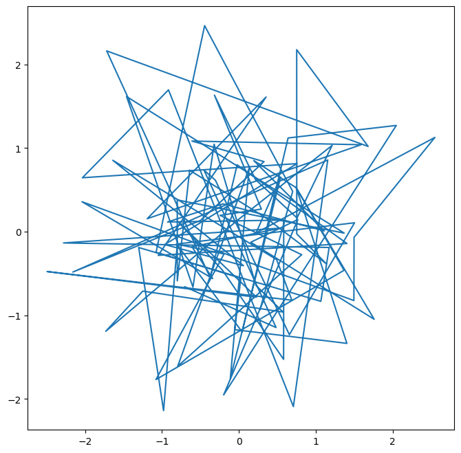
To create a scatterplot instead of a line plot, we can pass an additional argument to ax.plot() specifying the marker style. "o" indicates circles as markers.

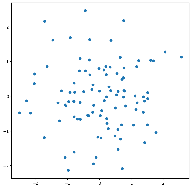
Alternatively, you can use the ax.scatter() function specifically for creating scatter plots.

Suppressing Output with Semicolons:

In Jupyter notebooks, the output of the last line of a cell is automatically displayed. Sometimes, you might not want to display text output from plotting commands (e.g., long lines of Matplotlib output). You can suppress this text output by ending the line with a semicolon ;. The semicolon does not prevent the plot from being displayed, it only suppresses text output.

Plot Labels and Titles:

To make plots informative, you should add labels to the axes and a title to the plot. You can use the ax.set_xlabel(), ax.set_ylabel(), and ax.set_title() methods for this.

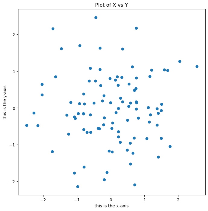
Modifying Figure Size:

You can change the size of an existing figure using the fig.set_size_inches() method.

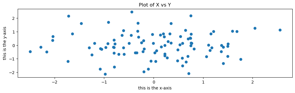
Multiple Plots in a Figure (Subplots):

You can create figures with multiple plots arranged in a grid using subplots(). The nrows and ncols keyword arguments specify the number of rows and columns of subplots.

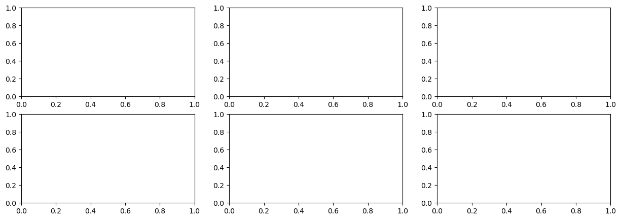
subplots(nrows=2, ncols=3) returns a figure object fig and an array of axes objects axes. axes is a 2x3 NumPy array where each element axes[i, j] corresponds to the axes object for the subplot in the i-th row and j-th column.

Saving Figures:

You can save figures to image files using the fig.savefig() method.

fig.savefig() takes the filename as the first argument. The dpi argument controls the resolution of the saved image (dots per inch). Higher DPI values result in higher resolution images.

Contour Plots:

Contour plots are used to visualize three-dimensional data in two dimensions. They represent surfaces by drawing contour lines (lines of constant value) on a 2D plane. ax.contour() creates contour plots. It typically takes three arguments: x-coordinates, y-coordinates, and a 2D array representing the z-values (heights) at each (x, y) point.

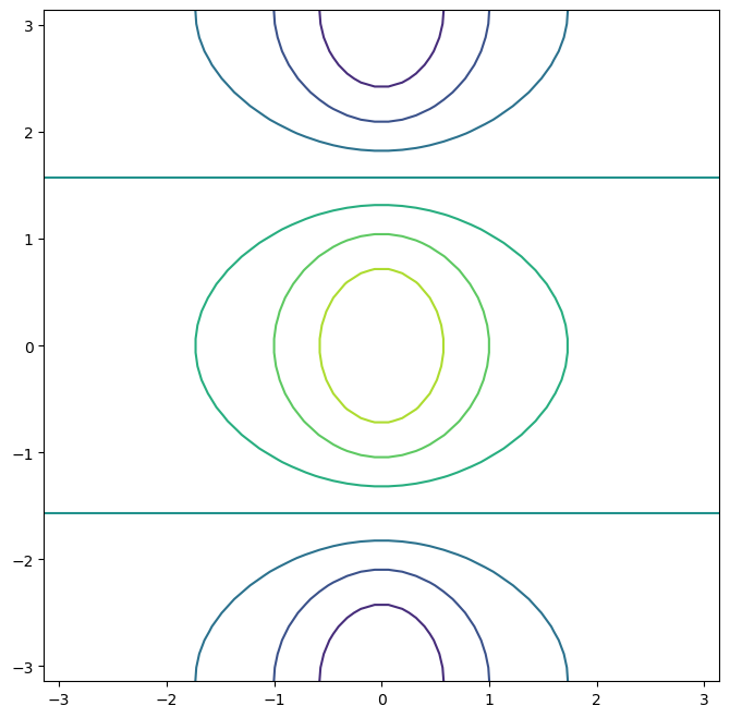
np.linspace(a, b, n) creates an array of n evenly spaced numbers from a to b. np.multiply.outer() calculates the outer product of two arrays.

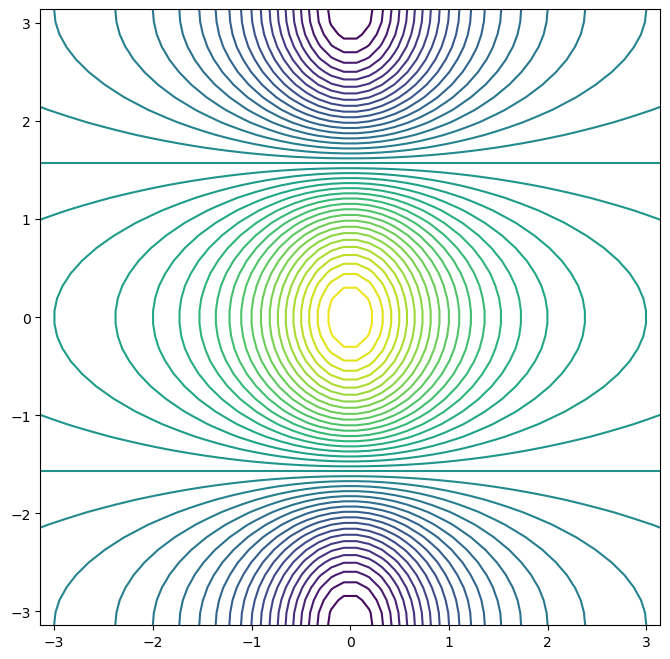
The levels argument controls the number of contour lines to be drawn.

Heatmaps (Image Plots):

Heatmaps or image plots represent data as a color-coded grid. ax.imshow() creates heatmaps. It takes a 2D array as input, and the color of each cell in the grid is determined by the corresponding value in the array.

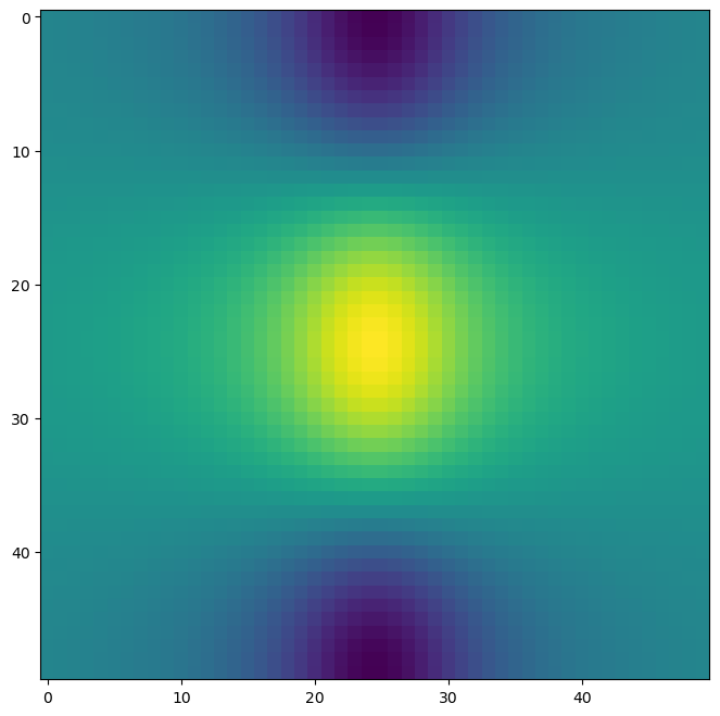
Matplotlib is a vast library with extensive capabilities for creating various types of plots and customizing their appearance. For more examples and options, explore the Matplotlib gallery: matplotlib.org/stable/gallery/index.html.

Sequences and Slice Notation¶

Python and NumPy extensively use the concept of sequences to represent ordered collections of data. We’ve already encountered lists and tuples as Python sequences, and NumPy arrays are also sequences. Slice notation is a powerful and concise way to access subsets or ranges of elements within sequences.

Creating Sequences:

NumPy provides functions to create numerical sequences easily.

np.linspace(start, stop, num) creates a sequence of num evenly spaced numbers between start and stop (inclusive).

np.arange(start, stop, step) creates a sequence of numbers starting from start, incrementing by step, and stopping before reaching stop (exclusive of stop). If step is not specified, it defaults to 1.

Slice Notation: Accessing Subsequences:

Slice notation uses square brackets [] and colons : to specify a range of indices. The general format is [start:stop:step].

• start: The starting index (inclusive, default is 0).
• stop: The ending index (exclusive).
• step: The step size or increment (default is 1).

In this example, [3:6] is a slice object (internally, it’s slice(3, 6)). It extracts characters from index 3 up to (but not including) index 6.

Understanding Slice Endpoints:

A key thing to remember about slice notation is that the stop index is exclusive. This is why np.arange(0, 10) produces numbers from 0 to 9, not including 10. Similarly, slice(3, 6) extracts elements at indices 3, 4, and 5, but not 6.

Slice Defaults:

If you omit start, it defaults to 0 (beginning of the sequence). If you omit stop, it defaults to the end of the sequence. If you omit step, it defaults to 1.

Slice notation is extremely versatile and is used extensively in Python and NumPy for accessing and manipulating parts of sequences. For more options and details on slice objects, see the documentation: slice?.

Indexing Data: Accessing Elements in Arrays and DataFrames¶

Indexing is the process of selecting specific elements or subsets of data from arrays, matrices, and data frames. We’ve already seen basic indexing with NumPy arrays. Let’s explore more advanced indexing techniques.

Creating a Sample Array:

Let’s create a 4x4 NumPy array to demonstrate indexing:

Basic Indexing: Single Element Access:

To access a single element in a 2D array A, use A[row_index, column_index]. Remember that indexing is zero-based.

Indexing Rows, Columns, and Submatrices:

Selecting Multiple Rows or Columns using Lists:

To select multiple rows, pass a list of row indices as the first index. To select all columns, use a colon : as the second index.

To select specific columns, pass a list of column indices as the second index and use : to select all rows.

Attempting to Select Submatrices Incorrectly:

A common mistake when trying to select a submatrix is to use two lists of indices directly:

This does not select the submatrix formed by rows 1 and 3 and columns 0 and 2. Instead, it performs element-wise indexing, returning a 1D array: [A[1,0], A[3,2]].

Correctly Selecting Submatrices:

To select a submatrix (a rectangular portion of the array), you need to use a combination of indexing techniques. One way is to chain indexing operations:

This first selects rows 1 and 3, creating an intermediate array. Then, from this intermediate array, it selects columns 0 and 2, resulting in the desired submatrix.

Using np.ix_() for Submatrix Selection:

NumPy’s np.ix_() function provides a more convenient and efficient way to select submatrices using lists of row and column indices. np.ix_() creates an “index mesh” that allows for proper submatrix indexing.

Submatrix Selection using Slices:

Slices are a very efficient way to select contiguous submatrices.

1:4:2 selects rows with indices 1 and 3 (start=1, stop=4, step=2). 0:3:2 selects columns with indices 0 and 2.

Why Slices Work for Submatrices, but Lists Don’t Directly:

Slices and lists are treated differently by NumPy indexing. Slices are designed for selecting contiguous ranges, making them naturally suited for submatrix selection. Lists, when used directly in multidimensional indexing (like A[[1,3],[0,2]]), are interpreted as index pairs for element-wise selection, not submatrix selection. np.ix_() bridges this gap by creating an index mesh that allows lists to be used for submatrix selection.

Boolean Indexing:

Boolean indexing is a powerful technique for selecting elements based on conditions. You create a Boolean array (an array of True and False values) and use it to index another array. Elements corresponding to True in the Boolean array are selected.

Now, keep_rows is a Boolean array: [False, True, False, True]. When used to index A, it selects the rows where keep_rows is True.

Boolean Indexing vs. Integer Indexing:

It’s important to distinguish between Boolean indexing and integer indexing. Even though np.array([0,1,0,1]) and keep_rows might seem numerically similar (if you treat True as 1 and False as 0), they behave differently in indexing.

Integer indexing with [0, 1, 0, 1] selects and repeats rows based on the integer indices. Boolean indexing with keep_rows selects rows where the corresponding Boolean value is True.

Boolean Indexing with np.ix_():

You can combine Boolean indexing with np.ix_() to select submatrices based on Boolean conditions for both rows and columns.

Mixing Lists and Boolean Arrays with np.ix_():

np.ix_() is flexible and allows you to mix lists of indices with Boolean arrays for submatrix selection.

NumPy’s indexing capabilities, including integer indexing, slice notation, Boolean indexing, and np.ix_(), provide powerful and versatile ways to access and manipulate data within arrays and matrices. Understanding these techniques is essential for efficient data analysis and manipulation in Python. For a comprehensive guide to NumPy indexing, refer to the NumPy tutorial.

Loading Data with Pandas¶

In data analysis, you often work with datasets stored in external files. Pandas is a powerful Python library specifically designed for data manipulation and analysis. It introduces the DataFrame, a tabular data structure that is highly effective for working with structured data.

DataFrames: Tabular Data in Pandas:

A Pandas DataFrame is like a table or a spreadsheet. It organizes data into rows and columns. Each column can have a different data type (numeric, string, datetime, etc.). DataFrames also have row and column labels (indices and column names), making it easy to access and manipulate data.

Reading Data from Files:

Pandas provides functions to read data from various file formats. pd.read_csv() is used to read data from CSV (Comma-Separated Values) files, which are a common format for storing tabular data.

pd.read_csv("Auto.csv") reads the data from the file “Auto.csv” (assuming it’s in the same directory as your notebook) and creates a DataFrame named Auto. Running Auto displays the DataFrame in a tabular format.

Reading Whitespace-Delimited Data:

Some data files use whitespace (spaces, tabs) as delimiters instead of commas. For these files, you can use pd.read_csv() with the delim_whitespace=True argument.

Handling Missing Values:

Data files often contain missing values, which are represented in various ways (e.g., NA, ?, blank spaces). When reading data, Pandas can automatically handle certain missing value representations. However, you might need to specify custom missing value indicators using the na_values argument in pd.read_csv().

Let’s examine the “horsepower” column in our Auto DataFrame:

The dtype of this column is object, which indicates that Pandas has interpreted the “horsepower” values as strings (text), not numbers. This is likely because there are non-numeric values in the column.

Let’s find the unique values in the “horsepower” column:

We see the value '?' in the unique values. It appears that '?' is used to represent missing values in the “horsepower” column. Pandas, by default, doesn’t recognize '?' as a missing value indicator.

To correctly handle '?' as missing values, we can use the na_values argument in pd.read_csv(). We tell Pandas to treat '?' as missing values, and Pandas will replace them with NaN (Not a Number), which is Pandas’ standard representation for missing values.

After specifying na_values=["?"], Pandas correctly reads '?' as missing values (NaN). Attempting to sum the “horsepower” column now might result in NaN because of the missing values.

DataFrame Shape:

The Auto.shape attribute of a DataFrame returns a tuple indicating the number of rows and columns: (rows, columns).

Handling Missing Data: Dropping Rows with Missing Values:

Pandas provides various ways to handle missing data. One simple approach is to remove rows that contain missing values using the dropna() method.

Auto.dropna() creates a new DataFrame Auto_new where rows with any NaN values are removed. The shape of Auto_new will be smaller than Auto if rows were dropped.

It’s common to overwrite the original DataFrame variable with the cleaned DataFrame after handling missing values.

DataFrame Columns:

The Auto.columns attribute gives you a list of column names in the DataFrame.

Pandas DataFrames are powerful tools for reading, cleaning, and manipulating tabular data. They provide efficient ways to handle missing values, select subsets of data, perform calculations, and much more. In the following sections, we’ll explore more DataFrame operations for data analysis.

Basics of Selecting Rows and Columns in DataFrames¶

Pandas DataFrames offer flexible ways to select and access rows and columns of data. Understanding these selection methods is crucial for data manipulation and analysis.

Accessing Columns:

You can access a single column of a DataFrame using square bracket notation [] with the column name as a string.

This returns a Pandas Series, which is a one-dimensional labeled array representing a single column of the DataFrame.

To access multiple columns, pass a list of column names within the square brackets.

This returns a new DataFrame containing only the specified columns.

Accessing Rows using Slices:

Similar to NumPy arrays and Python lists, you can use slice notation to select a range of rows from a DataFrame. When you use slice notation directly with a DataFrame (like Auto[:3]), it operates on the rows.

This returns a DataFrame containing the first three rows (rows with index 0, 1, and 2).

Accessing Rows using Boolean Indexing:

You can use a Boolean Series (a Series of True and False values) to select rows based on conditions.

This selects rows where the condition Auto["year"] > 80 is True.

DataFrame Index:

DataFrames have an index, which labels the rows. If you don’t explicitly set an index when reading data, Pandas automatically creates a default integer index starting from 0.

Setting DataFrame Index:

You can set a column of the DataFrame as the index using the set_index() method. This can be useful if you have a column with unique identifiers for each row (e.g., car names).

Auto.set_index("name") creates a new DataFrame Auto_re where the “name” column is now the index, and the “name” column itself is removed as a regular column.

Accessing Rows by Index Labels using .loc[]:

After setting an index, you can access rows using their index labels with the .loc[] indexer.

Auto_re.loc[rows] selects rows whose index labels are in the rows list.

Accessing Rows and Columns by Integer Position using .iloc[]:

The .iloc[] indexer allows you to access rows and columns based on their integer positions (0-based indices), regardless of the index labels.

.loc[] vs. .iloc[]:

• .loc[]: Primarily for label-based indexing. Use index labels (row names, column names) to select data.
• .iloc[]: Primarily for integer-position-based indexing. Use integer positions (0, 1, 2, ...) to select data, regardless of labels.

Duplicate Index Entries:

DataFrame indices don’t have to be unique. There can be multiple rows with the same index label.

If there are multiple rows with the same index label, .loc[] will return all of them.

More on Selecting Rows and Columns with Pandas¶

Let’s delve deeper into advanced row and column selection techniques in Pandas DataFrames.

Combining Boolean Indexing and Column Selection:

Suppose we want to select specific columns (weight and origin) for a subset of cars (those built after 1980). We can combine Boolean indexing for rows and column selection using .loc[].

Functional Row Selection with lambda Functions and .loc[]:

Pandas .loc[] indexer can accept functions (often lambda functions) as row or column selectors. Lambda functions are small, anonymous functions defined inline. They are useful for creating concise functions for filtering or transforming data.

lambda df: df["year"] > 80 defines an anonymous function that takes a DataFrame df as input and returns a Boolean Series df["year"] > 80. .loc[] then uses this Boolean Series to select rows from Auto_re.

Combining Multiple Conditions with & (and) and | (or):

You can combine multiple conditions in Boolean indexing using the & (and) and | (or) operators. Remember to enclose each condition in parentheses () for correct operator precedence.

String-Based Filtering with .str.contains():

For DataFrames with string indices or columns, you can use string methods like .str.contains() for filtering based on string patterns.

Suppose we want to select “Ford” and “Datsun” cars with displacement less than 300. We can use .str.contains() on the DataFrame index (which is “name” in Auto_re) to check if the car name contains “ford” or “datsun”.

df.index.str.contains("ford") applies the string method .contains("ford") to each element of the DataFrame index (car names). It returns a Boolean Series indicating whether each index label contains “ford”. Similarly for df.index.str.contains("datsun"). We use | (or) to combine these conditions.

Summary of DataFrame Indexing:

Pandas DataFrames offer a rich set of indexing methods for selecting rows and columns:

• Column Selection: DataFrame["column_name"], DataFrame[["col1", "col2"]]
• Row Selection (Slices): DataFrame[start_row:end_row]
• Row Selection (Boolean Indexing): DataFrame[Boolean_Series]
• Label-based Indexing (.loc[]): DataFrame.loc[row_labels, column_labels]
• Integer-position-based Indexing (.iloc[]): DataFrame.iloc[row_positions, column_positions]
• Functional Row/Column Selection (.loc[] with lambda functions): DataFrame.loc[lambda df: condition, column_selectors]
• Combining Conditions (&, |)
• String-based Filtering (.str.contains(), etc.)

Mastering these indexing techniques is essential for effectively working with and analyzing data using Pandas DataFrames.

For Loops: Repeating Operations¶

For loops are fundamental control flow structures in programming. They allow you to repeatedly execute a block of code for each item in a sequence (like a list, tuple, string, or range). For loops are essential for automating repetitive tasks and processing collections of data.

Basic For Loop Structure:

The basic syntax of a for loop in Python is:

The for loop iterates through each item in the sequence. In each iteration, the variable is assigned the current item, and the code inside the indented block (the loop body) is executed.

Example: Summing List Elements:

In this loop:

1. total is initialized to 0.
2. The loop iterates through the list [3, 2, 19].
3. In the first iteration, value is assigned 3, and total becomes 0 + 3 = 3.
4. In the second iteration, value is assigned 2, and total becomes 3 + 2 = 5.
5. In the third iteration, value is assigned 19, and total becomes 5 + 19 = 24.
6. After the loop finishes, the final value of total (24) is printed.

Nested For Loops:

You can nest for loops inside each other to iterate over multiple sequences.

In this nested loop, the inner loop runs completely for each iteration of the outer loop. For each value in [2, 3, 19], the inner loop iterates through all weight values in [3, 2, 1].

Increment Notation (+=, -=, *=, /=):

Python provides shorthand increment operators like +=, -=, *=, /=. a += b is equivalent to a = a + b. These operators are often more concise and can be slightly more efficient in some cases.

Using zip() to Iterate over Multiple Sequences Simultaneously:

The zip() function is useful for iterating over multiple sequences in parallel. It combines corresponding elements from multiple sequences into tuples.

zip([2, 3, 19], [0.2, 0.3, 0.5]) creates an iterator that yields tuples: (2, 0.2), (3, 0.3), (19, 0.5). The for loop unpacks each tuple into value and weight variables in each iteration.

String Formatting: Creating Dynamic Strings:

String formatting is used to create strings dynamically by inserting values of variables into strings. Python offers several string formatting methods. One common method is using f-strings (formatted string literals), introduced in Python 3.6.

f-strings:

f-strings are created by prefixing a string literal with f or F. You can embed expressions inside f-strings by enclosing them in curly braces {}. The expressions are evaluated, and their values are inserted into the string.

.format() method:

Another string formatting method is using the .format() method of strings. You use placeholders {} within the string and pass the values to be inserted as arguments to .format(). Placeholders can be numbered (e.g., {0}, {1}) to refer to arguments by position.

{0} refers to the first argument passed to .format() (column_name), and {1:.2%} refers to the second argument (missing_percent) formatted as a percentage with 2 decimal places.

Example: Looping through DataFrame Columns and Printing Missing Percentages:

Let’s create a DataFrame with some missing values and loop through its columns to print the percentage of missing values in each column.

In this loop:

1. D.columns gives a list of column names in DataFrame D.
2. The loop iterates through each col (column name).
3. np.isnan(D[col]) checks for NaN (missing values) in the column D[col] and returns a Boolean Series (True for NaN, False otherwise).
4. .mean() on the Boolean Series calculates the proportion of True values (which is the fraction of missing values).
5. template.format(col, np.isnan(D[col]).mean()) formats the string using the column name and the calculated missing percentage.
6. print() displays the formatted string for each column.

For loops and string formatting are essential tools in Python for automating tasks, processing data, and generating informative output. For more advanced string formatting options, refer to the Python string formatting documentation: docs.python.org/3/library/string.html.

Additional Graphical and Numerical Summaries with Pandas¶

Pandas integrates well with Matplotlib, providing convenient methods for creating plots directly from DataFrames. Pandas also offers built-in methods for generating numerical summaries of data.

Plotting DataFrames Directly:

Pandas DataFrames have .plot attribute, which provides access to various plotting methods. You can create plots directly from DataFrame columns using these methods.

Scatter Plots with DataFrame.plot.scatter():

The DataFrame.plot.scatter(x, y) method creates a scatter plot with the column specified by x on the x-axis and the column specified by y on the y-axis.

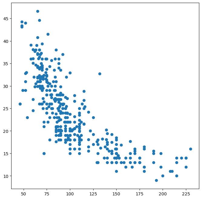
To plot DataFrame columns directly by name, you can use Auto.plot.scatter():

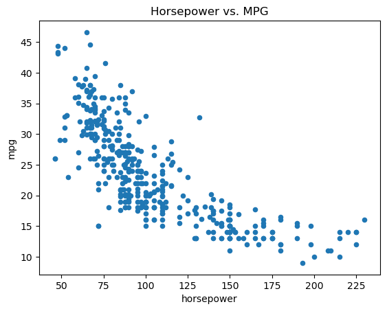
Auto.plot.scatter("horsepower", "mpg") creates a scatter plot of “mpg” vs. “horsepower” from the Auto DataFrame. It returns the Matplotlib axes object (ax), which you can then use to customize the plot further (e.g., set title, labels).

Accessing Figure from Axes:

If you have an axes object ax and want to save the entire figure containing it, you can access the figure object using ax.figure.

Plotting to a Specific Axes:

You can instruct Pandas plotting methods to draw on a specific Matplotlib axes object using the ax= argument. This is useful when you want to place plots within a grid of subplots.

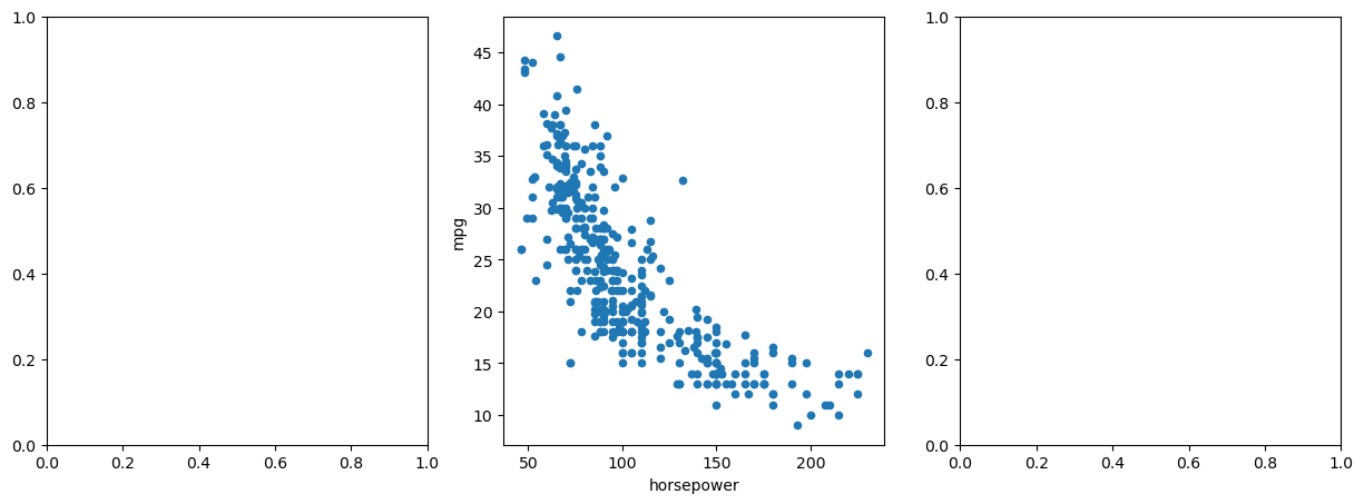
Accessing DataFrame Columns as Attributes:

You can access DataFrame columns not only using square bracket notation (Auto["horsepower"]) but also as attributes using dot notation (Auto.horsepower).

Treating Categorical Variables: astype('category'):

Sometimes, numerical columns represent categorical variables (e.g., “cylinders” in the Auto dataset). You might want to treat them as categorical for certain analyses or visualizations. You can convert a column to categorical type using astype('category') or pd.Series(column, dtype="category").

Box Plots with DataFrame.boxplot():

Box plots are useful for visualizing the distribution of a numerical variable for different categories. DataFrame.boxplot(column, by) creates box plots of the column variable, grouped by the categories in the by column.

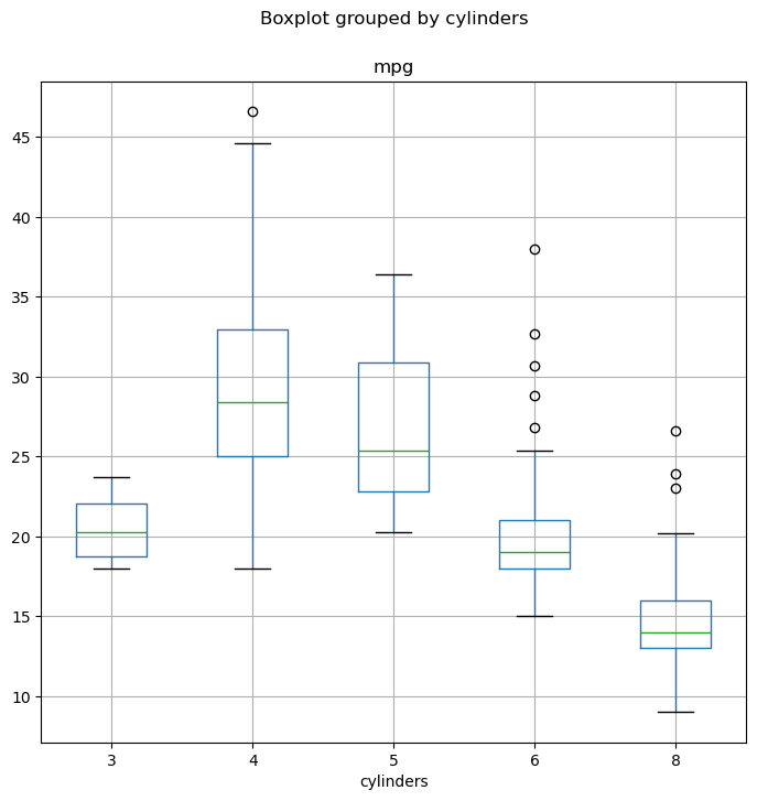
Histograms with DataFrame.hist():

Histograms visualize the distribution of a numerical variable by dividing the data into bins and showing the frequency of data points in each bin. DataFrame.hist(column) creates a histogram of the column variable.

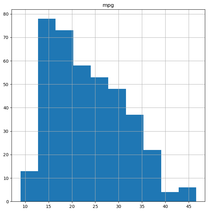
You can customize histograms using arguments like color and bins.

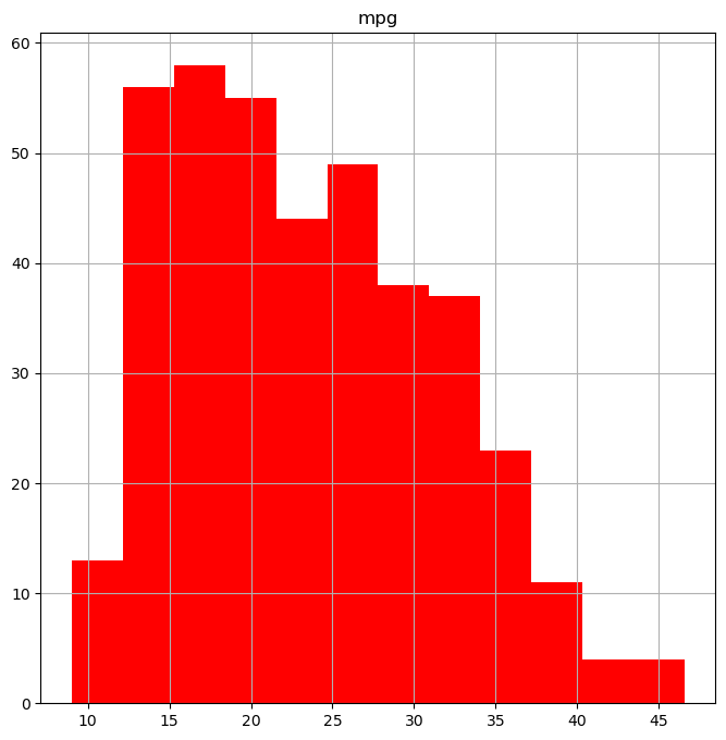
Scatterplot Matrices with pd.plotting.scatter_matrix():

Scatterplot matrices are useful for visualizing pairwise relationships between multiple variables. pd.plotting.scatter_matrix(DataFrame) creates a matrix of scatter plots for all pairs of numerical columns in the DataFrame.

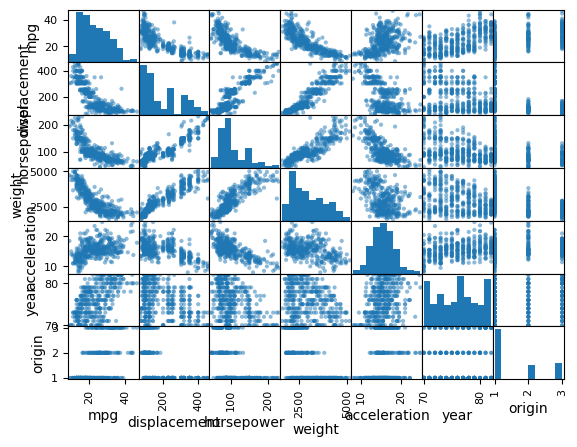
You can create scatterplot matrices for a subset of columns by passing a list of column names.

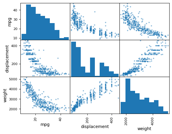
Numerical Summaries with DataFrame.describe() and Series.describe():

The DataFrame.describe() method provides descriptive statistics (count, mean, std, min, 25%, 50%, 75%, max) for each numerical column in a DataFrame.

You can also use .describe() on a single column (Pandas Series) to get descriptive statistics for that column.

Pandas provides a rich set of tools for data visualization and numerical summarization, making it a powerful library for exploratory data analysis and data understanding.

Exiting Jupyter Notebook:

To exit Jupyter Notebook, go to the “File” menu in the Jupyter Notebook interface and select “Shut Down”. This will shut down the Jupyter server and close the notebook.

Congratulations on completing this introduction to Python for data science! You’ve learned fundamental Python concepts, explored NumPy for numerical computing, Matplotlib for plotting, and Pandas for data manipulation and analysis. These are essential building blocks for your journey into data science with Python. Continue practicing and exploring these libraries to deepen your skills.