Linear Regression

Importing packages¶

We begin by importing essential Python libraries that will be used throughout this notebook. It’s standard practice to group imports at the beginning for better organization and readability.

New imports¶

As we progress through this lab and explore more advanced techniques, we’ll introduce new functions and libraries. To highlight these additions and maintain code clarity, we import them upfront in this section. This practice makes it easier to quickly understand which new tools are being utilized in each part of the lab. Keeping imports near the top of a notebook enhances readability, allowing anyone reviewing the code to quickly grasp the dependencies.

We will provide detailed explanations of these functions as they become relevant in the notebook.

Python offers flexibility in importing modules. Instead of importing an entire module, we can selectively import specific objects, such as functions or classes. This is beneficial for keeping the namespace clean and avoiding potential naming conflicts. We will leverage specific objects from the statsmodels package, importing them individually as needed.

To improve the readability of long import statements, we can use a line break \ to split them across multiple lines. This is especially helpful when importing several items from the same module.

We will also utilize custom functions specifically designed for the labs in this book, which are conveniently packaged in the ISLP package.

Renaming ModelSpec to MS using as MS is a common practice to shorten frequently used names, making the code cleaner and less verbose.

Inspecting Objects and Namespaces¶

Understanding namespaces and the objects within them is crucial for effective Python programming. The dir() function is a valuable tool for inspecting the contents of a namespace. It provides a list of all objects currently available in the specified namespace.

Executing dir() at the top level will display all objects accessible in the current global namespace. This includes built-in functions, imported modules, and any variables defined so far. Objects like __builtins__ are special namespaces containing references to Python’s built-in functions, such as print(), len(), etc.

Every Python object, whether it’s a variable, a function, or a module, has its own namespace. We can also use dir() to inspect the namespace of a specific object. This reveals the attributes and methods associated with that object. For example, let’s examine the namespace of a NumPy array:

The output of dir(A) will list all attributes and methods of the NumPy array A. You should see 'sum' in the listing, indicating that A.sum is a valid method for this array object. To learn more about the sum method, you can use Python’s help functionality by typing A.sum? in a code cell and executing it.

This will compute and display the sum of the elements in the array A.

Simple Linear Regression¶

In this section, we will delve into simple linear regression, a fundamental statistical technique. We’ll learn how to construct model matrices, also known as design matrices, using the ModelSpec() transform from the ISLP.models module. These matrices are essential for fitting linear regression models.

We will work with the well-known Boston housing dataset, which is included in the ISLP package. This dataset contains information on medv (median house value) for 506 neighborhoods in the Boston area. Our goal is to build a regression model that predicts medv using 13 predictor variables. These predictors include features like rm (average number of rooms per house), age (proportion of owner-occupied units built prior to 1940), and lstat (percentage of households with low socioeconomic status). We will employ the statsmodels package, a powerful Python library that provides implementations of various regression methods, for this task.

The ISLP package provides a convenient function load_data() to load datasets for the labs. Let’s load the Boston dataset and inspect its columns:

To understand the dataset in more detail, you can type Boston? in a code cell and execute it. This will display the dataset’s documentation, providing information about each variable.

We will start by fitting a simple linear regression model using the sm.OLS() function from statsmodels. Our response variable will be medv, and we will use lstat as our single predictor. For this simple model with only one predictor, we can manually create the model matrix X.

Here, we create a Pandas DataFrame X. The first column, “intercept”, consists of ones, representing the intercept term in the linear regression model. The second column, “lstat”, contains the values of the lstat predictor variable from the Boston dataset. X[:4] displays the first four rows of the model matrix, showing the structure of our design matrix.

Next, we extract the response variable y (median house value medv) and fit the linear regression model using sm.OLS().

It’s important to note that sm.OLS() only specifies the model. The actual model fitting is performed by the model.fit() method. The fit() method estimates the model coefficients by minimizing the sum of squared residuals. The result of model.fit() is stored in the results object, which contains all the information about the fitted model.

To get a concise summary of the fitted model, including parameter estimates, standard errors, t-statistics, and p-values, we can use the summarize() function from the ISLP package. This function takes the results object as input and returns a formatted summary table.

This output provides key information about the simple linear regression model, allowing us to assess the significance and direction of the relationship between lstat and medv.

Before exploring more ways to work with fitted models, let’s introduce a more versatile and general approach for constructing model matrices using transformations. This approach will be particularly useful when dealing with more complex models.

Using Transformations: Fit and Transform¶

In the previous example, creating the model matrix X was straightforward because we only had one predictor. However, in real-world scenarios, we often work with models containing multiple predictors, possibly with transformations, interactions, or polynomial terms. Manually constructing model matrices in such cases can become cumbersome and error-prone.

The sklearn package and the ISLP.models module introduce the concept of a transform to streamline this process. A transform is an object that encapsulates a specific data transformation. It’s initialized with parameters defining the transformation and has two primary methods: fit() and transform().

We will use the ModelSpec() transform from ISLP.models (renamed MS() for brevity) to define our model and construct the model matrix. ModelSpec() creates a transform object. Then, the fit() and transform() methods are applied sequentially to generate the corresponding model matrix.

Let’s demonstrate this process for our simple linear regression model with lstat as the predictor in the Boston dataset. We create a transform object using design = MS(['lstat']).

The fit() method is applied to the original dataset. It performs any necessary initial computations based on the transform specification. For instance, it might calculate means and standard deviations for centering and scaling variables, or in our case, it checks if the specified variable 'lstat' exists in the Boston DataFrame. The transform() method then applies the fitted transformation to the data and produces the model matrix.

In this simple case, the fit() method performs minimal operations. It primarily verifies the presence of the 'lstat' variable in the Boston DataFrame. Then, transform() constructs the model matrix X with two columns: an ‘intercept’ column and the lstat variable itself.

The fit() and transform() operations can be combined into a single step using the fit_transform() method. This is often more convenient.

As before, the design object is modified after the fit() operation, storing information about the fitted transformation. The true power of this pipeline will become evident as we build more complex models involving interactions and transformations in later sections.

Let’s return to our fitted regression model (results). The results object has numerous methods and attributes for performing inference and analysis. We’ve already used summarize() for a concise summary. For a comprehensive and detailed summary of the fit, we can use the summary() method.

This provides a wealth of information about the fitted model, including goodness-of-fit statistics, hypothesis tests, and detailed coefficient information.

The estimated coefficients of the fitted model can be accessed through the params attribute of the results object.

This will output a Pandas Series containing the estimated intercept and slope coefficients for our simple linear regression model.

The get_prediction() method is used to obtain predictions from the fitted model. It can also generate confidence intervals and prediction intervals for the predicted values of medv for given values of lstat.

First, we create a new Pandas DataFrame, new_df, containing the values of lstat at which we want to make predictions.

We then use the transform() method of our design object to create the model matrix newX corresponding to these new lstat values. This ensures that the new data is transformed in the same way as the original data used to fit the model.

Next, we use the get_prediction() method of the results object, passing newX as input, to compute predictions. We can access the predicted mean values using the predicted_mean attribute.

This will output the predicted medv values for lstat values of 5, 10, and 15, based on our fitted linear regression model.

To obtain confidence intervals for the predicted values, we use the conf_int() method of the new_predictions object. We specify the desired confidence level using the alpha parameter (e.g., alpha=0.05 for 95% confidence intervals).

This will provide the 95% confidence intervals for the mean predicted medv values at the specified lstat values. These intervals represent the uncertainty in estimating the average medv for a given lstat.

Prediction intervals, which are wider than confidence intervals, account for the additional uncertainty in predicting an individual medv value. To compute prediction intervals, we set obs=True in the conf_int() method.

For example, for an lstat value of 10, the 95% confidence interval for the predicted mean medv is (24.47, 25.63), while the 95% prediction interval for an individual medv is (12.82, 37.28). As expected, both intervals are centered around the same predicted value (25.05 for medv when lstat is 10), but the prediction interval is significantly wider due to the added uncertainty of predicting a single observation.

Now, let’s visualize the relationship between medv and lstat by creating a scatter plot using DataFrame.plot.scatter(). We will then add the fitted regression line to this plot to visualize the linear relationship.

Defining Functions¶

While the ISLP package provides utilities for plotting, let’s take this opportunity to define our own function for adding a regression line to an existing plot. This will illustrate how to define custom functions in Python and enhance our plotting capabilities.

Let’s break down the function definition:

• def abline(ax, b, m): defines a function named abline that takes three arguments: ax (an axis object from matplotlib), b (the intercept), and m (the slope).
• The docstring """Add a line with slope m and intercept b to axis ax""" describes what the function does. Good documentation is crucial for making code understandable.
• xlim = ax.get_xlim() retrieves the current x-axis limits of the plot associated with the axis object ax.
• ylim = [m * xlim[0] + b, m * xlim[1] + b] calculates the y-coordinates of the line at the left and right x-axis limits using the equation of a line: y = mx + b.
• ax.plot(xlim, ylim) plots the line on the specified axis ax using the calculated x and y coordinates.

To make our abline function more versatile, we can add the ability to pass additional plotting arguments, such as line color, style, and width, directly to the underlying ax.plot() function. We can achieve this using *args and **kwargs.

• *args allows the function to accept any number of positional arguments (arguments without names), which are then passed directly to ax.plot().
• **kwargs allows the function to accept any number of keyword arguments (arguments with names, like linewidth=3), which are also passed to ax.plot().

This enhancement makes our abline function more flexible, allowing us to customize the appearance of the regression line. For a deeper understanding of function definitions, refer to the Python documentation on defining functions: docs.python.org/tutorial.

Let’s use our newly defined abline function to add the regression line to a scatter plot of medv vs. lstat.

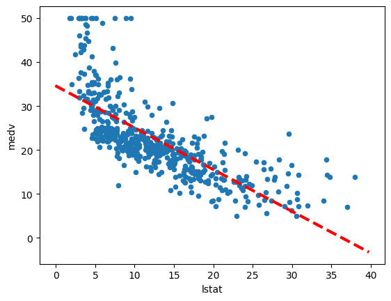
• ax = Boston.plot.scatter("lstat", "medv") creates a scatter plot of lstat on the x-axis and medv on the y-axis using Pandas’ plotting capabilities. The resulting axis object is stored in ax.
• abline(ax, results.params[0], results.params[1], "r--", linewidth=3) calls our abline function to add the regression line to the plot.
  • ax is the axis object of our scatter plot.
  • results.params[0] is the estimated intercept from our fitted regression model.
  • results.params[1] is the estimated slope from our fitted regression model.
  • "r--" is a format string that specifies a red dashed line.
  • linewidth=3 sets the line width to 3 pixels.

The call to ax.plot() within abline becomes ax.plot(xlim, ylim, 'r--', linewidth=3), incorporating the additional plotting arguments. The resulting plot will show the scatter points and the red dashed regression line. Observing the plot, we might notice some evidence of non-linearity in the relationship between lstat and medv, suggesting that a simple linear model might not fully capture the relationship. We will explore non-linear models later in this lab.

While matplotlib does offer a built-in function ax.axline() to add lines to plots, knowing how to write custom functions like abline empowers us to create more specialized and expressive visualizations.

Next, we will examine diagnostic plots to assess the adequacy of our linear regression model. These plots, discussed in detail in Section 3.3 of the ISLP textbook, help us identify potential problems with the model assumptions. We will look at residual plots and leverage plots.

We can obtain the fitted values and residuals from our fitted model as attributes of the results object. Influence measures, which help identify influential observations, can be computed using the get_influence() method.

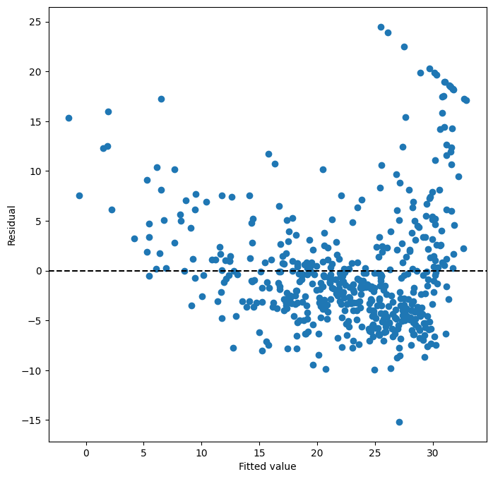
• ax = subplots(figsize=(8, 8))[1] creates a figure and a set of subplots. subplots() returns a tuple containing the figure and a list of axes objects. We use [1] to select the second element of the tuple, which is the axes object we need for our plot. figsize=(8, 8) sets the size of the figure in inches.
• ax.scatter(results.fittedvalues, results.resid) generates a scatter plot with the fitted values on the x-axis and the residuals on the y-axis. results.fittedvalues and results.resid are attributes of the results object containing the fitted values and residuals, respectively.
• ax.set_xlabel("Fitted value") and ax.set_ylabel("Residual") set the labels for the x and y axes.
• ax.axhline(0, c="k", ls="--") adds a horizontal line at y=0 to the plot. c="k" sets the color to black, and ls="--" sets the line style to dashed. This horizontal line helps to visually assess whether the residuals are randomly scattered around zero, as expected for a good model.

Based on the residual plot, we can look for patterns or deviations from randomness. In this case, we might observe some curvature, further suggesting potential non-linearity in the relationship between lstat and medv.

Leverage statistics quantify the influence of each observation on the regression model. They can be computed using the hat_matrix_diag attribute of the object returned by the get_influence() method.

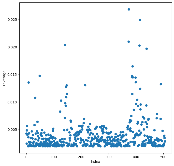
• infl = results.get_influence() calculates various influence measures for each observation in the dataset. The result is stored in the infl object.
• ax = subplots(figsize=(8, 8))[1] creates a figure and axes for the leverage plot, similar to the residual plot.
• ax.scatter(np.arange(X.shape[0]), infl.hat_matrix_diag) creates a scatter plot of leverage values against the observation index. infl.hat_matrix_diag is an attribute of the infl object containing the diagonal elements of the hat matrix, which represent the leverage of each observation. np.arange(X.shape[0]) creates an array of indices from 0 to the number of observations minus 1, which we use as x-coordinates for the plot.
• ax.set_xlabel("Index") and ax.set_ylabel("Leverage") label the axes.
• np.argmax(infl.hat_matrix_diag) finds the index of the observation with the largest leverage value. np.argmax() returns the index of the maximum value in an array. Identifying high leverage points can be important for understanding which observations have the most influence on the regression model.

By examining the leverage plot, we can identify observations with unusually high leverage. These observations may warrant further investigation as they can disproportionately affect the regression results.

Multiple Linear Regression¶

Now, let’s extend our analysis to multiple linear regression, where we use more than one predictor variable to model the response. To fit a multiple linear regression model using ordinary least squares, we again utilize the ModelSpec() transform to construct the model matrix and specify the response variable. The ModelSpec() transform is quite flexible in how it accepts model specifications. In this case, providing a list of column names is sufficient. We will fit a model with two predictors: lstat and age.

Notice how we’ve combined the model matrix construction into a concise single line using MS(["lstat", "age"]).fit_transform(Boston). This demonstrates the efficiency of the ModelSpec() approach.

The Boston dataset contains 12 predictor variables. Typing all of them individually to fit a model with all predictors would be tedious. We can use a shorthand to include all predictor variables in the model.

• Boston.columns gives us a Pandas Index object containing all column names of the Boston DataFrame.
• Boston.columns.drop("medv") drops the column name “medv” from this index, effectively giving us a list of all predictor variable names. This list is stored in the terms variable.

Now we can fit a multiple linear regression model including all variables in terms as predictors.

This code fits a multiple linear regression model using all available predictors in the Boston dataset. The summarize(results) output will show the coefficients, standard errors, t-statistics, and p-values for each predictor in the model.

What if we want to perform a regression using almost all variables, but exclude one or a few specific predictors? For instance, in the previous regression output, the age predictor might have a high p-value, suggesting it might not be a significant predictor in the model. We might want to refit the model excluding age. We can easily do this using the drop() method again.

• Boston.columns.drop(["medv", "age"]) drops both “medv” and “age” from the column names, resulting in a list of predictor variables excluding age.
• The rest of the code proceeds as before, fitting and summarizing the multiple linear regression model without the age predictor.

Multivariate Goodness of Fit¶

After fitting a multiple linear regression model, we often want to assess the overall goodness of fit. Key metrics for this include $R^2$ (R-squared) and RSE (Residual Standard Error). We can access these and other components of the fitted model directly from the results object.

We can explore the attributes of the results object using dir(results). This will show us all available attributes and methods. For example, results.rsquared gives us the R-squared value, and np.sqrt(results.scale) gives us the RSE. results.scale is the estimate of the error variance, so taking its square root gives us the RSE.

Variance Inflation Factors (VIFs) are useful for detecting multicollinearity in the predictor variables of a regression model. High VIF values indicate that a predictor variable is highly correlated with other predictors, which can inflate the variance of the coefficient estimates and make interpretation difficult. We will calculate VIFs for our multiple regression model and use this as an opportunity to introduce the concept of list comprehension in Python.

List Comprehension¶

List comprehension is a concise and powerful way to create lists in Python. It provides a more readable and often more efficient alternative to traditional for loops for building lists. Python also supports dictionary and generator comprehensions, but we will focus on list comprehension here.

Let’s say we want to compute the VIF for each predictor variable in our model matrix X. We have a function variance_inflation_factor() (imported as VIF) from statsmodels.stats.outliers_influence that does this. It takes two arguments: the model matrix and the index of the predictor variable column.

• vals = [VIF(X, i) for i in range(1, X.shape[1])] is the list comprehension. Let’s break it down:
  • for i in range(1, X.shape[1]): This is the loop part. It iterates over the column indices of X from 1 to X.shape[1]-1. We start from index 1 to exclude the intercept column (column 0) when calculating VIFs, as VIF is not typically calculated for the intercept. X.shape[1] gives the number of columns in X.
  • VIF(X, i): For each index i in the loop, this calculates the VIF for the i-th predictor variable using the VIF() function.
  • [ ... ]: The square brackets enclose the entire expression, indicating that we are building a list. The result of each VIF(X, i) calculation is added to this list.
• vif = pd.DataFrame({"vif": vals}, index=X.columns[1:]) creates a Pandas DataFrame to neatly display the VIF values.
  • {"vif": vals} creates a dictionary where the key is “vif” and the value is the list of VIF values vals. This dictionary is used to create a DataFrame with a column named “vif”.
  • index=X.columns[1:] sets the index of the DataFrame to be the column names of X starting from the second column (index 1), which are the predictor variable names (excluding the intercept column name).

The resulting vif DataFrame will show the VIF value for each predictor variable in the model. Generally, VIF values greater than 5 or 10 are considered indicative of significant multicollinearity. In this particular example with the Boston dataset, the VIFs might not be excessively high, but in other datasets, they can be more concerning.

The list comprehension approach is often more concise and readable than writing an equivalent for loop. The code above using list comprehension is functionally equivalent to the following for loop:

List comprehension provides a more streamlined way to perform such repetitive operations, making the code cleaner and easier to understand.

Interaction Terms¶

In many real-world scenarios, the effect of one predictor variable on the response might depend on the value of another predictor variable. This is known as an interaction effect. We can easily include interaction terms in our linear models using ModelSpec().

To include an interaction term between two variables, say lstat and age, we include a tuple ("lstat", "age") in the list of terms passed to ModelSpec().

• MS(["lstat", "age", ("lstat", "age")]) specifies that we want to include the main effects of lstat and age, as well as their interaction term. The tuple ("lstat", "age") tells ModelSpec() to create an interaction term by multiplying lstat and age.
• The rest of the code proceeds as before, fitting and summarizing the model. The summarize() output will now include a row for the interaction term lstat:age, showing its estimated coefficient, standard error, t-statistic, and p-value.

By including interaction terms, we allow for more flexible models that can capture more complex relationships between predictors and the response.

Non-linear Transformations of the Predictors¶

Linear regression assumes a linear relationship between the predictors and the response. However, in many cases, the true relationship might be non-linear. We can extend linear regression to model non-linear relationships by including non-linear transformations of the predictors in the model matrix.

The ModelSpec() transform is flexible and allows us to include various types of terms beyond just column names and interactions. For example, we can use the poly() function from ISLP.models to include polynomial terms of a predictor variable.

• poly("lstat", degree=2) specifies that we want to include polynomial terms of lstat up to degree 2. This will create columns for lstat and lstat^2 (and an intercept, which is implicitly added by MS()).
• MS([poly("lstat", degree=2), "age"]) includes the quadratic polynomial terms for lstat and the main effect of age in the model matrix.
• The summarize() output will now show coefficients for the linear term of lstat (labeled poly(lstat, degree=2)[1]) and the quadratic term of lstat (labeled poly(lstat, degree=2)[2]), as well as for age.

The p-value associated with the quadratic term of lstat (the third row in the summarize() output) can indicate whether adding a quadratic term significantly improves the model fit compared to a linear model. A very small p-value suggests that the quadratic term is indeed important and that the relationship between lstat and medv is non-linear.

By default, poly() creates a basis matrix of orthogonal polynomials. Orthogonal polynomials are designed to improve the numerical stability of least squares computations, especially when dealing with higher-degree polynomials. Under the hood, poly() is a wrapper for the Poly() function in ISLP.models, which performs the actual basis matrix construction.

If we wanted to use simple raw polynomials (i.e., lstat and lstat**2 directly), we could have included the argument raw=True in the poly() call: poly("lstat", degree=2, raw=True). In this case, the basis matrix would consist of columns for lstat and lstat**2. Although the basis matrices would be different, both orthogonal and raw polynomial bases represent the same space of quadratic polynomials, so the fitted values and model predictions would be identical; only the interpretation of the coefficients would change. By default, poly() does not include an intercept column in its output because MS() automatically adds an intercept column to the model matrix.

To formally compare the linear model (results1) and the quadratic model (results3), we can use the anova_lm() function to perform an analysis of variance (ANOVA) test. ANOVA helps us determine if the improvement in fit from adding the quadratic term is statistically significant.

• anova_lm(results1, results3) compares the nested models results1 (linear model with lstat and age) and results3 (quadratic model with lstat, lstat^2, and age). The first argument should be the simpler (nested) model, and subsequent arguments should be increasingly complex models.
• The ANOVA output will show an F-statistic and a p-value. The null hypothesis is that the larger model (quadratic model) does not provide a significantly better fit than the smaller model (linear model). The alternative hypothesis is that the larger model is significantly better. A small p-value (typically less than 0.05) rejects the null hypothesis, indicating that the larger model provides a statistically significant improvement in fit.

In this case, the F-statistic is 177.28, and the associated p-value is essentially zero. This provides strong evidence that the quadratic polynomial term in lstat significantly improves the linear model. This is consistent with our earlier observation of non-linearity in the relationship between medv and lstat. In this specific case, the F-statistic from ANOVA is the square of the t-statistic for the quadratic term in the summarize(results3) output. This is because the two models differ by only one degree of freedom (the quadratic term).

The anova_lm() function can compare more than two nested models. When given multiple models, it compares each successive pair of models. This explains why there are NaN values in the first row of the ANOVA output, as there is no model preceding the first one for comparison.

Let’s examine the residual plot for the quadratic model to see if the non-linearity issue has been addressed.

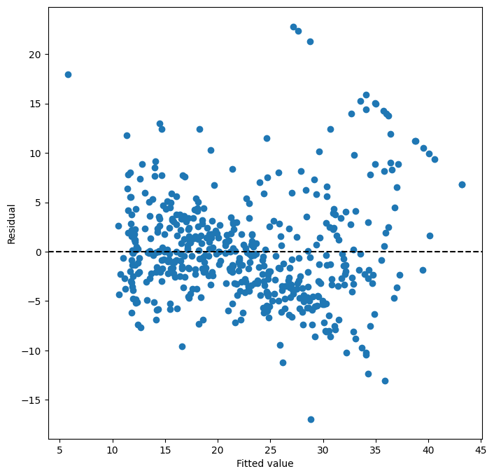
By examining the residual plot for the quadratic model, we hope to see a more random scatter of residuals around zero, with no discernible patterns. This would suggest that the quadratic model provides a better fit and captures the non-linearity in the data more effectively.

To fit cubic or higher-degree polynomial models, we can simply change the degree argument in the poly() function call. For example, poly("lstat", degree=3) would include cubic polynomial terms.

Qualitative Predictors¶

So far, we have primarily focused on quantitative predictor variables. However, many datasets also include qualitative or categorical predictors. Let’s explore how to handle qualitative predictors in linear regression using the Carseats dataset, which is included in the ISLP package. We will try to predict Sales (child car seat sales) in 400 locations based on various predictors.

The Carseats dataset includes qualitative predictors like ShelveLoc, which indicates the quality of the shelving location within a store where car seats are displayed. ShelveLoc can take on three values: Bad, Medium, and Good.

When ModelSpec() encounters a qualitative variable like ShelveLoc, it automatically generates dummy variables (also known as one-hot encoding). Dummy variables are numerical representations of categorical variables, allowing them to be used in regression models. For a categorical variable with $k$ levels, ModelSpec() will typically create $k-1$ dummy variables. These dummy variables are often referred to as a one-hot encoding of the categorical feature. In one-hot encoding, for each category (except one, which serves as the baseline), a new binary variable is created. If an observation belongs to that category, the dummy variable is 1; otherwise, it is 0. The category that is omitted (the baseline) is implicitly represented when all dummy variables are 0.

In the case of ShelveLoc with levels Bad, Medium, and Good, ModelSpec() will create two dummy variables. By default, it drops the first level alphabetically (which is Bad in this case) to avoid multicollinearity with the intercept. So, we will see dummy variables for ShelveLoc[Good] and ShelveLoc[Medium]. ShelveLoc[Good] will be 1 if the shelving location is “Good” and 0 otherwise. ShelveLoc[Medium] will be 1 if the location is “Medium” and 0 otherwise. When both ShelveLoc[Good] and ShelveLoc[Medium] are 0, it implies that the shelving location is “Bad” (the baseline category).

Let’s fit a multiple regression model using the Carseats dataset, including some interaction terms.

• allvars = list(Carseats.columns.drop("Sales")) gets a list of all column names in Carseats except for “Sales”, which is our response variable.
• final = allvars + [("Income", "Advertising"), ("Price", "Age")] defines the list of terms to be included in the model. It starts with all main effects from allvars and then adds two interaction terms: ("Income", "Advertising") (interaction between Income and Advertising) and ("Price", "Age") (interaction between Price and Age).
• X = MS(final).fit_transform(Carseats) creates the model matrix based on the specified terms. ModelSpec() will automatically handle the qualitative variable ShelveLoc by creating dummy variables.
• The rest of the code fits and summarizes the model.

In the regression output from summarize(model.fit()), you will see coefficients for ShelveLoc[Good] and ShelveLoc[Medium]. The coefficient for ShelveLoc[Good] represents the estimated difference in sales between a store with a “Good” shelving location and a store with a “Bad” shelving location (holding other predictors constant). A positive coefficient for ShelveLoc[Good] indicates that, on average, stores with good shelving locations tend to have higher sales compared to stores with bad shelving locations. Similarly, the coefficient for ShelveLoc[Medium] represents the difference in sales between “Medium” and “Bad” shelving locations. By comparing the coefficients of ShelveLoc[Good] and ShelveLoc[Medium], we can understand the relative impact of different shelving locations on car seat sales.