Advanced time series regression requires careful attention to asymptotic theory, non-stationarity, and high persistence in economic data. This chapter extends the foundational concepts from Chapter 10, examining conditions under which OLS maintains desirable properties with time series data, characterizing highly persistent processes including random walks, and developing transformation methods such as first differencing to address non-stationarity and avoid spurious regression results.
The development proceeds hierarchically through increasingly sophisticated concepts. We establish asymptotic properties of OLS under stationary and weakly dependent time series processes (Section 11.1), examine the implications of trending data and spurious regression problems (Section 11.2), characterize integrated processes of order one I(1) including random walks and their properties (Section 11.3), introduce first differencing as a transformation method to induce stationarity (Section 11.4), and analyze differenced regression models including interpretation of coefficients and dynamic multipliers (Section 11.5). Throughout, we emphasize both theoretical foundations and practical implementation using Python for macroeconomic applications.
# %pip install matplotlib numpy pandas statsmodels wooldridge scipy -qimport matplotlib.pyplot as plt
import numpy as np
import pandas as pd
import statsmodels.formula.api as smf
import wooldridge as wool
from scipy import (
stats, # Used here for generating random numbers from specific distributions
)11.1 Asymptotics with Time Series
The properties of OLS estimators (like consistency and asymptotic normality) rely on certain assumptions about the underlying time series processes. In time series, the assumption of random sampling (MLR.2/SLR.2) is replaced by assumptions about the stationarity and weak dependence of the series.
Key Time Series Assumptions:
Stationarity (TS.1’): A time series is (covariance) stationary if:
for all (constant mean)
for all (constant variance)
depends only on , not on (autocovariances depend only on the time gap)
Stationarity ensures the time series process is “stable” over time, with no trends or time-varying volatility. This replaces the cross-sectional random sampling assumption.
Weak Dependence (TS.2’): A time series is weakly dependent if the correlation between observations diminishes sufficiently quickly as the time distance between them increases. Formally, as at a sufficiently fast rate.
Weak dependence ensures that observations far apart in time are nearly independent. This is crucial for applying versions of the Law of Large Numbers and Central Limit Theorem to time series data.
Zero Conditional Mean (TS.3’): for all .
This is the time series analog of MLR.4. It requires the error to be uncorrelated with current and all past values of regressors, but allows for correlation between and future values (weaker than strict exogeneity).
Asymptotic Properties: Under appropriate stationarity, weak dependence, and zero conditional mean conditions (along with homoscedasticity for standard errors), OLS estimators in time series regressions are:
Consistent: as
Asymptotically Normal: as
This allows for standard inference (t-tests, F-tests) with dependent time series data, provided the sample size is large enough. When serial correlation is present, standard errors must be corrected (see Chapter 12).
Example 11.4: Efficient Markets Hypothesis (EMH)
The Efficient Markets Hypothesis (EMH), in its weak form, suggests that current asset prices fully reflect all information contained in past price movements. A key implication is that past returns should not predict future returns. We can test this by regressing a stock return series on its own lagged values. If the EMH holds, the coefficients on the lagged returns should be zero.
We use the nyse dataset containing daily returns for the New York Stock Exchange index.
# Load the NYSE daily returns data
nyse = wool.data("nyse")
# Rename the 'return' column to 'ret' for convenience in formulas
# Note: Wooldridge dataset 'nyse' has a column 'return', but 'return' is a python keyword.
# Renaming avoids potential issues or needing Q() in formulas.
nyse["ret"] = nyse["return"]

# Create lagged variables for the return series up to 3 lags
# lag 1: ret_{t-1}
# lag 2: ret_{t-2}
# lag 3: ret_{t-3}
nyse["ret_lag1"] = nyse["ret"].shift(1)
nyse["ret_lag2"] = nyse["ret"].shift(2)
nyse["ret_lag3"] = nyse["ret"].shift(3)

# Define and estimate three regression models:
# Model 1: Regress ret_t on ret_{t-1}
# Model 2: Regress ret_t on ret_{t-1} and ret_{t-2}
# Model 3: Regress ret_t on ret_{t-1}, ret_{t-2}, and ret_{t-3}
reg1 = smf.ols(formula="ret ~ ret_lag1", data=nyse)
reg2 = smf.ols(formula="ret ~ ret_lag1 + ret_lag2", data=nyse)
reg3 = smf.ols(formula="ret ~ ret_lag1 + ret_lag2 + ret_lag3", data=nyse)

# Fit the models
results1 = reg1.fit()
results2 = reg2.fit()
results3 = reg3.fit()

# Display regression results for Model 1
table1 = pd.DataFrame(
    {
        "b": round(results1.params, 4),
        "se": round(results1.bse, 4),
        "t": round(results1.tvalues, 4),
        "pval": round(results1.pvalues, 4),
    },
)
# --- Regression 1: ret ~ ret_lag1 ---
table1  # Display regression results

# Interpretation (Model 1):
# The coefficient on the first lag (ret_lag1) is 0.0589. While small, it is not statistically
# significant (p-value = 0.122). This provides little evidence against the strict form of the EMH,
# suggesting that knowing yesterday's return provides limited predictive power for today's return.# Display regression results for Model 2
table2 = pd.DataFrame(
{
"b": round(results2.params, 4),
"se": round(results2.bse, 4),
"t": round(results2.tvalues, 4),
"pval": round(results2.pvalues, 4),
},
)
# --- Regression 2: ret ~ ret_lag1 + ret_lag2 ---
table2 # Display regression results
# Interpretation (Model 2):
# Adding the second lag (ret_lag2), we see its coefficient (-0.0381) is not statistically
# significant (p=0.319). The coefficient on the first lag remains similar (0.0603) and not significant (p=0.115).
# An F-test for the joint significance of both lags would be appropriate here.# Display regression results for Model 3
table3 = pd.DataFrame(
{
"b": round(results3.params, 4),
"se": round(results3.bse, 4),
"t": round(results3.tvalues, 4),
"pval": round(results3.pvalues, 4),
},
)
# --- Regression 3: ret ~ ret_lag1 + ret_lag2 + ret_lag3 ---
table3 # Display regression results
# Interpretation (Model 3):
# With three lags, none of the individual lag coefficients are statistically significant
# at the 5% level (p-values are 0.109, 0.293, 0.422).
# An F-test for joint significance (H0: coefficients on all three lags are zero) would
# provide a more definitive test of predictability based on the first three lags.
# Overall, the evidence for predictability based on multiple lags appears weak,
# consistent with the EMH, although transaction costs might negate any small predictable patterns.11.2 The Nature of Highly Persistent Time Series
Many economic time series, particularly levels of variables like GDP, price indices, or asset prices, exhibit high persistence. This means that shocks (unexpected changes) have lasting effects, and the series tends to wander far from its mean over time. Such series are often non-stationary.
A classic example of a highly persistent, non-stationary process is the Random Walk:
where is a zero-mean, uncorrelated (often assumed independent) shock term (also called white noise). The value today is simply the value yesterday plus a random shock. This means the effect of a shock persists indefinitely in future values of . Random walks are also called unit root processes or integrated of order 1 (I(1)) processes.
The following simulation generates and plots multiple realizations of a simple random walk ().
# Set a seed for reproducibility of the random numbers
np.random.seed(1234567)

# Initialize the plot settings
x_range = np.linspace(0, 50, num=51)  # Time periods 0 to 50
plt.figure(figsize=(10, 6))  # Make the plot a bit larger
plt.ylim([-18, 18])  # Set y-axis limits
plt.xlim([0, 50])  # Set x-axis limits

# Simulate and plot 30 independent random walk paths
for r in range(30):
    # Generate 51 standard normal shocks (mean 0, variance 1)
    e = stats.norm.rvs(0, 1, size=51)

    # Set the first shock to 0, implying y_0 = 0 (starting point)
    e[0] = 0

    # Create the random walk path by taking the cumulative sum of shocks
    # y_t = e_1 + e_2 + ... + e_t (since y_0 = 0)
    y = np.cumsum(e)

    # Add the path to the plot with light grey color
    plt.plot(x_range, y, color="lightgrey", linestyle="-")

# Add a horizontal line at y=0 for reference
plt.axhline(0, linewidth=2, linestyle="--", color="black")
plt.ylabel("y (Value of the process)")
plt.xlabel("Time")
plt.title("Simulated Random Walk Processes (without drift)")
plt.grid(True, linestyle="--", alpha=0.6)
plt.show()

# Observation: The paths wander widely and do not revert to a mean value (here, 0).
# The variance increases over time. This illustrates the non-stationary nature of a random walk.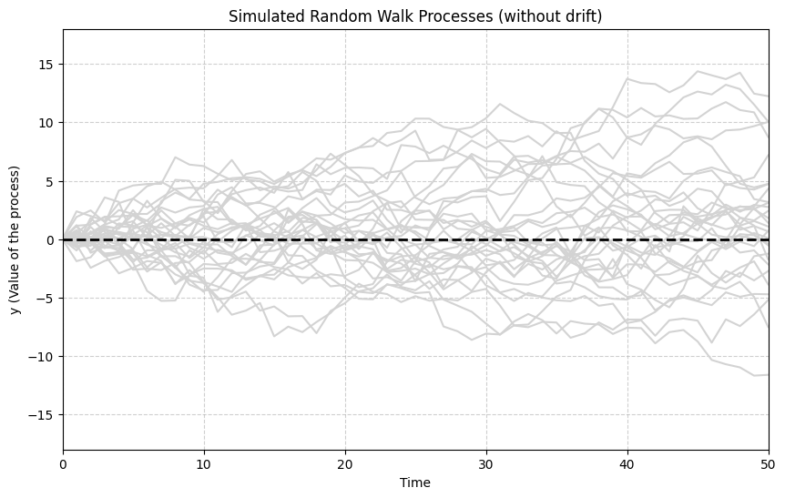
A Random Walk with Drift includes a constant term (), causing the series to trend upwards or downwards over time:
Taking the cumulative sum, . The series now has a linear time trend () plus the random walk component.
The next simulation shows random walks with a positive drift ().
# Reset the seed for reproducibility
np.random.seed(1234567)

# Initialize plot settings
x_range = np.linspace(0, 50, num=51)
plt.figure(figsize=(10, 6))
plt.ylim([0, 150])  # Adjusted ylim to accommodate drift
plt.xlim([0, 50])

# Simulate and plot 30 random walk paths with drift = 2
for r in range(30):
    # Generate standard normal shocks
    e = stats.norm.rvs(0, 1, size=51)
    e[0] = 0  # For y_0 = 0

    # Create the random walk path with drift by summing shocks and adding the drift component
    # y_t = y_0 + alpha*t + cumsum(e)
    # Here, alpha = 2, y_0 = 0
    y = np.cumsum(e) + 2 * x_range  # 2*x_range represents the drift term alpha*t

    # Add path to plot
    plt.plot(x_range, y, color="lightgrey", linestyle="-")

# Plot the deterministic drift line y = 2*t for reference
plt.plot(
    x_range,
    2 * x_range,
    linewidth=2,
    linestyle="--",
    color="black",
    label="Drift line (y=2t)",
)
plt.ylabel("y (Value of the process)")
plt.xlabel("Time")
plt.title("Simulated Random Walk Processes with Drift (alpha=2)")
plt.legend()
plt.grid(True, linestyle="--", alpha=0.6)
plt.show()

# Observation: The paths now exhibit a clear upward trend, determined by the drift term (alpha=2).
# They still wander randomly around this trend line due to the cumulative shocks.
# This type of process is also non-stationary (I(1)).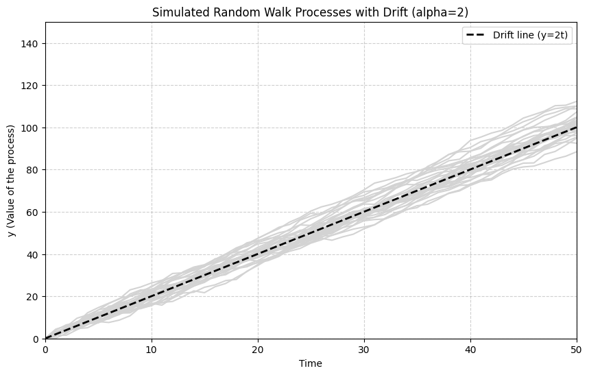
11.3 Differences of Highly Persistent Time Series
A key property of I(1) processes (like random walks with or without drift) is that their first difference is stationary (I(0)). The first difference, denoted , is simply the change in the series from one period to the next:
For a random walk , the first difference is . Since is assumed to be white noise (stationary), the first difference is stationary.
For a random walk with drift , the first difference is . This is also stationary, fluctuating around a mean of .
The following simulation shows the first differences of the random walks with drift generated previously.
# Reset the seed
np.random.seed(1234567)

# Initialize plot settings
x_range = np.linspace(1, 50, num=50)  # Time periods 1 to 50 for the differences
plt.figure(figsize=(10, 6))
plt.ylim([-3, 7])  # Adjusted ylim based on alpha + e_t (mean 2)
plt.xlim([0, 50])

# Simulate and plot first differences of 30 random walks with drift = 2
for r in range(30):
    # Generate shocks e_1, ..., e_50 (we need 51 points for y, 50 for diff)
    e = stats.norm.rvs(0, 1, size=51)
    # No need to set e[0]=0 if we calculate y directly with drift
    # Construct y_t = y_0 + alpha*t + cumsum(e), assume y_0=0, alpha=2
    # A slightly more direct way to get the difference: Dy_t = alpha + e_t
    # Note: the simulation below uses cumsum(2+e), which gives y_t = sum_{i=1}^t (2+e_i).
    # Then Dy_t = y_t - y_{t-1} = (2+e_t). This is equivalent.
    y = np.cumsum(
        2 + e,
    )  # Generates y_1, ..., y_51 with drift 2, starting implicitly from y_0=0

    # Calculate the first difference: Delta y_t = y_t - y_{t-1} for t=1,...,50
    # This gives 50 difference values.
    Dy = y[1:51] - y[0:50]  # Difference uses elements 1 to 50 and 0 to 49

    # Add the difference series to the plot
    plt.plot(x_range, Dy, color="lightgrey", linestyle="-")

# Add a horizontal line at the mean of the difference (alpha = 2)
plt.axhline(
    y=2,
    linewidth=2,
    linestyle="--",
    color="black",
    label="Mean difference (alpha=2)",
)
plt.ylabel("Delta y (First Difference)")
plt.xlabel("Time")
plt.title("First Differences of Simulated Random Walks with Drift (alpha=2)")
plt.legend()
plt.grid(True, linestyle="--", alpha=0.6)
plt.show()

# Observation: The first difference series (Delta y) now appears stationary. The paths fluctuate
# around a constant mean (alpha = 2) and do not exhibit the wandering behavior or trend seen
# in the levels (y). The variance seems constant over time. This illustrates how differencing
# can transform a non-stationary I(1) process into a stationary I(0) process.
11.4 Regression with First Differences
Regressing one I(1) variable on another can lead to spurious regression: finding a statistically significant relationship (high R-squared, significant t-stats) even when the variables are truly unrelated, simply because both are trending over time due to their I(1) nature.
One common approach to avoid spurious regression when dealing with I(1) variables is to estimate the regression model using first differences. If the original model is:
and both and are I(1), we can difference the equation to get:
(Note: The intercept differences out if it represents a constant level. If the original model included a time trend, differencing would result in a constant term in the differenced equation.)
If and are stationary (I(0)), then OLS estimation of the differenced equation yields valid results. The coefficient retains its interpretation as the effect of a change in on .
Example 11.6: Fertility Equation
Let’s revisit the relationship between the general fertility rate (gfr) and the real value of the personal exemption (pe) from the fertil3 dataset. Both gfr and pe might be I(1) processes. We estimate the relationship using first differences.
# Load the fertil3 data
fertil3 = wool.data("fertil3")
T = len(fertil3)

# Define yearly time index
fertil3.index = pd.date_range(start="1913", periods=T, freq="YE").year

# Compute first differences of gfr and pe using pandas .diff() method
# .diff(1) calculates the difference between an element and the previous element.
fertil3["gfr_diff1"] = fertil3["gfr"].diff()
fertil3["pe_diff1"] = fertil3["pe"].diff()

# Display the first few rows showing the original variables and their differences
# Note that the first row of the differenced variables will be NaN (Not a Number).
# First few rows with differenced variables:
# Display first few rows with differenced variables
fertil3[["gfr", "pe", "gfr_diff1", "pe_diff1"]].head()Now, we regress the first difference of gfr on the first difference of pe. statsmodels automatically drops rows with NaN values, so the first observation is excluded.
# Estimate the linear regression using first differences
# Delta(gfr_t) = beta_0 + beta_1 * Delta(pe_t) + error_t
# Note: The intercept here (beta_0) represents the average annual change in gfr
# NOT accounted for by changes in pe. It captures any underlying linear trend in gfr.
reg1 = smf.ols(formula="gfr_diff1 ~ pe_diff1", data=fertil3)
results1 = reg1.fit()

# Display the regression results
table1 = pd.DataFrame(
    {
        "b": round(results1.params, 4),
        "se": round(results1.bse, 4),
        "t": round(results1.tvalues, 4),
        "pval": round(results1.pvalues, 4),
    },
)
# --- Regression in First Differences: Delta(gfr) ~ Delta(pe) ---
table1  # Display regression results

# Interpretation (Differenced Model):
# The coefficient on Delta(pe) (pe_diff1) is -0.0427 and is not statistically significant (p=0.137).
# This suggests that a $1 increase in the change of the personal exemption from one year
# to the next is associated with a decrease of about 0.04 points in the change of the
# fertility rate in the same year. This differs from the results obtained using levels in Chapter 10,
# highlighting how accounting for persistence can change conclusions.
# The intercept (-0.7848) suggests a slight downward trend in gfr after accounting for changes in pe.We can also include lags of the differenced explanatory variable, similar to an FDL model but applied to differences.
# Create lagged first differences of pe
fertil3["pe_diff1_lag1"] = fertil3["pe_diff1"].shift(1)
fertil3["pe_diff1_lag2"] = fertil3["pe_diff1"].shift(2)

# Estimate the regression with current and lagged first differences of pe
# Delta(gfr_t) = beta_0 + delta_0*Delta(pe_t) + delta_1*Delta(pe_{t-1}) + delta_2*Delta(pe_{t-2}) + error_t
reg2 = smf.ols(
    formula="gfr_diff1 ~ pe_diff1 + pe_diff1_lag1 + pe_diff1_lag2",
    data=fertil3,
)
results2 = reg2.fit()

# Display the regression results
table2 = pd.DataFrame(
    {
        "b": round(results2.params, 4),
        "se": round(results2.bse, 4),
        "t": round(results2.tvalues, 4),
        "pval": round(results2.pvalues, 4),
    },
)
# --- Regression with Lagged First Differences ---
# Dependent Variable: Delta(gfr)
table2  # Display regression results

# Interpretation (Lagged Differences):
# - The contemporaneous effect (pe_diff1) is -0.0362 (p=0.181), not significant.
# - The first lag (pe_diff1_lag1) has a coefficient of -0.0140 (p=0.614), insignificant.
# - The second lag (pe_diff1_lag2) has a coefficient of 0.1100 (p<0.001), highly significant.
# These results suggest that changes in the personal exemption have a delayed effect on changes
# in the fertility rate, with the strongest impact appearing two years later.
# This differs from the FDL model in levels (Example 10.4), showing a positive effect at lag 2.
# The Long-Run Propensity (LRP) in this differenced model would be estimated by summing the delta coefficients.This chapter established essential principles for applying OLS to time series: the critical importance of stationarity and weak dependence for valid asymptotic inference, the distinct characteristics of highly persistent integrated I(1) processes including random walks, and the use of first differencing as a systematic technique to induce stationarity and avoid spurious regression problems. These foundations prepare for more advanced time series methods in subsequent chapters.