Chapter 9: Specification and Data Issues

Learning Objectives

Upon completion of this chapter, readers will demonstrate proficiency in specification testing and data quality analysis using Python by:

9.1 Conducting RESET tests for functional form misspecification using statsmodels diagnostic functions with fitted value polynomials.

9.2 Implementing Davidson-MacKinnon tests for comparing non-nested regression models using statsmodels hypothesis testing framework.

9.3 Detecting and analyzing measurement error bias in regression coefficients through simulation studies with NumPy random number generation.

9.4 Handling proxy variables for unobserved explanatory variables by including available substitutes in statsmodels OLS regressions.

9.5 Computing least absolute deviations (LAD) regression as a robust alternative to OLS using statsmodels QuantReg with median regression.

9.6 Identifying influential observations and outliers using standardized residuals, leverage statistics, and Cook’s distance in statsmodels influence diagnostics.

9.7 Analyzing missing data patterns and implementing listwise deletion or imputation strategies using pandas missing data functions.

9.8 Visualizing functional form diagnostics through partial residual plots and component-plus-residual plots using statsmodels graphics.

9.9 Comparing OLS and robust regression results to assess sensitivity of conclusions to outliers and non-normality.

Regression analysis beyond the basic OLS assumptions requires careful attention to several critical issues. This chapter addresses five key challenges that arise in empirical econometric work: functional form specification, measurement error in variables, missing data patterns, influential outliers, and robust estimation methods. Each issue can substantially affect coefficient estimates, standard errors, and statistical inference if not properly addressed.

The organization follows a hierarchical development from foundational concepts to advanced applications. We begin with functional form misspecification and formal tests (Section 9.1), examine the distinct consequences of measurement error in dependent versus explanatory variables (Section 9.2), analyze missing data mechanisms and their implications (Section 9.3), identify and handle outlying observations (Section 9.4-9.5), and conclude with two important extensions: proxy variables for unobserved factors (Section 9.6) and models with random coefficients (Section 9.7).

Throughout this chapter, we demonstrate theoretical results through simulation studies and illustrate practical applications using real econometric datasets. The chapter concludes with comprehensive guidance on diagnostic procedures and decision frameworks for applied research.

# %pip install matplotlib numpy pandas statsmodels wooldridge scipy -q

import matplotlib.pyplot as plt
import numpy as np
import pandas as pd
import statsmodels.api as sm
import statsmodels.formula.api as smf
import statsmodels.stats.outliers_influence as smo  # For RESET test and outlier diagnostics
import wooldridge as wool
from IPython.display import display
from scipy import stats  # For generating random numbers

9.1 Functional Form Misspecification¶

Assumption MLR.1 from Chapter 3 requires correct specification of the population regression function. When the true relationship between variables is non-linear but we impose a linear specification, or when we omit important interaction terms, coefficient estimates become biased and inconsistent. This section develops formal tests for detecting functional form misspecification and presents methods for comparing alternative specifications.

Consequences of misspecification. Using an incorrect functional form creates several problems: (i) biased coefficient estimates, since omitted non-linear terms act as omitted variables; (ii) invalid inference, as standard errors and test statistics assume correct specification; (iii) poor out-of-sample predictions, particularly when extrapolating beyond the observed range; and (iv) incorrect marginal effects and economic interpretation.

Testing strategy. We consider two complementary approaches: the RESET test for detecting general misspecification within a given model, and the Davidson-MacKinnon J-test for comparing non-nested alternative specifications. Both tests are straightforward to implement and provide valuable diagnostic information about model adequacy.

9.1.1 The RESET Test¶

The Regression Specification Error Test, developed by Ramsey (1969), provides a general test for functional form misspecification. The test augments the original regression with powers of the fitted values and tests their joint significance. If these polynomial terms are significant, they indicate that the original specification fails to capture important non-linearities in the data.

Test construction. Consider the baseline model:

y = \beta_0 + \beta_1 x_1 + \cdots + \beta_k x_k + u

(1)

Estimate this model by OLS and obtain fitted values $\hat{y}_i$ . The RESET test estimates the augmented regression:

y = \beta_0 + \beta_1 x_1 + \cdots + \beta_k x_k + \delta_2 \hat{y}^2 + \delta_3 \hat{y}^3 + \text{error}

(2)

and tests the joint hypothesis $H_0: \delta_2 = \delta_3 = 0$ using an F-test. Under the null hypothesis of correct specification, the F-statistic follows an F-distribution with $(q, n-k-q-1)$ degrees of freedom, where $q$ is the number of polynomial terms added (typically 2).

Intuition. If the original model omits squares, cubes, or interactions of the $x$ variables, these may be partially captured by $\hat{y}^2$ and $\hat{y}^3$ , since $\hat{y}$ is a linear combination of the regressors. Significant coefficients on these terms signal that additional functional form flexibility is needed.

9.1.2 Example: Housing Price Equation¶

We apply the RESET test to the housing price model from Chapter 8. The baseline specification regresses house price (in thousands of dollars) on lot size, square footage, and number of bedrooms. This linear specification imposes constant marginal effects and rules out interaction terms or non-linearities in these relationships.

# RESET Test Implementation: Detecting Functional Form Misspecification
# The test adds powers of fitted values to detect omitted nonlinearities

# Load housing price data
hprice1 = wool.data("hprice1")

# Dataset info
data_info = pd.DataFrame(
    {
        "Metric": ["Number of houses", "Number of variables"],
        "Value": [hprice1.shape[0], hprice1.shape[1]],
    },
)
data_info

# Step 1: Estimate the baseline linear model
# This is our null hypothesis specification
baseline_model = smf.ols(
    formula="price ~ lotsize + sqrft + bdrms",
    data=hprice1,
)
baseline_results = baseline_model.fit()

# Baseline model summary
baseline_summary = pd.DataFrame(
    {
        "Metric": ["Dependent variable", "R-squared", "Adjusted R-squared"],
        "Value": [
            "price (house price in $1000s)",
            f"{baseline_results.rsquared:.4f}",
            f"{baseline_results.rsquared_adj:.4f}",
        ],
    },
)
baseline_summary

# Step 2: Generate polynomial terms from fitted values
# Theory: If model is misspecified, powers of y_hat capture omitted terms
hprice1["fitted_sq"] = baseline_results.fittedvalues**2  # y_hat^2
hprice1["fitted_cub"] = baseline_results.fittedvalues**3  # y_hat^3

# RESET test construction details
reset_info = pd.DataFrame(
    {
        "Component": ["Original predictors", "Added test terms", "H_0", "H_1"],
        "Description": [
            "lotsize, sqrft, bdrms",
            "fitted^2, fitted^3",
            "Coefficients on fitted^2 and fitted^3 = 0 (no misspecification)",
            "At least one polynomial term != 0 (misspecification present)",
        ],
    },
)
reset_info

# Step 3: Estimate augmented regression with polynomial terms
augmented_reset = smf.ols(
    formula="price ~ lotsize + sqrft + bdrms + fitted_sq + fitted_cub",
    data=hprice1,
)
augmented_results = augmented_reset.fit()

# Display auxiliary regression results with interpretation
reset_table = pd.DataFrame(
    {
        "Variable": augmented_results.params.index,
        "Coefficient": augmented_results.params.round(4),
        "Std_Error": augmented_results.bse.round(4),
        "t_stat": augmented_results.tvalues.round(3),
        "p_value": augmented_results.pvalues.round(4),
        "Test_Term": ["No", "No", "No", "No", "YES", "YES"],  # Mark RESET test terms
    },
)

# Display RESET auxiliary regression results
display(reset_table)

# 4. Perform an F-test for the joint significance of the added terms
# H0: Coefficients on fitted_sq and fitted_cub are both zero.
hypotheses = ["fitted_sq = 0", "fitted_cub = 0"]
ftest_man = augmented_results.f_test(hypotheses)
fstat_man = ftest_man.statistic  # Extract F-statistic value
fpval_man = ftest_man.pvalue

# RESET Test (Manual F-Test)
reset_manual = pd.DataFrame(
    {
        "Method": ["Manual F-Test"],
        "F-statistic": [f"{fstat_man:.4f}"],
        "p-value": [f"{fpval_man:.4f}"],
    },
)
reset_manual

# Interpretation (Manual RESET): The F-statistic is 4.6682 and the p-value is 0.0120.
# Since the p-value is less than 0.05, we reject the null hypothesis.
# This suggests that the original linear model suffers from functional form misspecification.
# Non-linear terms (perhaps logs, squares, or interactions) might be needed.

statsmodels also provides a convenient function for the RESET test.

# Reload data if needed
hprice1 = wool.data("hprice1")

# Estimate the original linear regression again
reg = smf.ols(formula="price ~ lotsize + sqrft + bdrms", data=hprice1)
results = reg.fit()

# Perform automated RESET test using statsmodels.stats.outliers_influence
# Pass the results object and specify the maximum degree of the fitted values to include (degree=3 means ^2 and ^3)
# --- RESET Test (Automated) ---
reset_output = smo.reset_ramsey(res=results, degree=3)
fstat_auto = reset_output.statistic
fpval_auto = reset_output.pvalue

# RESET Test Results (Automated)
pd.DataFrame(
    {
        "Metric": ["RESET F-statistic", "RESET p-value"],
        "Value": [f"{fstat_auto:.4f}", f"{fpval_auto:.4f}"],
    },
)

# Interpretation (Automated RESET): The automated test yields the same F-statistic (4.6682)
# and p-value (0.0120), confirming the rejection of the null hypothesis and indicating
# functional form misspecification in the linear model.

Non-nested Tests (Davidson-MacKinnon)¶

When we have two competing, non-nested models (meaning neither model is a special case of the other), we can use tests like the Davidson-MacKinnon test to see if one model provides significant explanatory power beyond the other.

The test involves augmenting one model (Model 1) with the fitted values from the other model (Model 2). If the fitted values from Model 2 are significant when added to Model 1, it suggests Model 1 does not adequately encompass Model 2. The roles are then reversed.

Possible outcomes: Neither model rejected, one rejected, both rejected.

Here, we compare the linear housing price model (Model 1) with a log-log model (Model 2).

# Reload data if needed
hprice1 = wool.data("hprice1")

# Define the two competing, non-nested models:
# Model 1: Linear levels model
reg1 = smf.ols(formula="price ~ lotsize + sqrft + bdrms", data=hprice1)
results1 = reg1.fit()

# Model 2: Log-log model (except for bdrms)
reg2 = smf.ols(
    formula="price ~ np.log(lotsize) +np.log(sqrft) + bdrms",
    data=hprice1,
)
results2 = reg2.fit()

# --- Davidson-MacKinnon Test (Implementation via encompassing model F-test) ---
# An alternative way to perform these tests is to create a comprehensive model
# that includes *all* non-redundant regressors from both models.
# Then, test the exclusion restrictions corresponding to each original model.

# Comprehensive model including levels and logs (where applicable)
reg3 = smf.ols(
    formula="price ~ lotsize + sqrft + bdrms + np.log(lotsize) + np.log(sqrft)",
    data=hprice1,
)
results3 = reg3.fit()

# Test Model 1 vs Comprehensive Model:
# H0: Coefficients on np.log(lotsize) and np.log(sqrft) are zero (i.e., Model 1 is adequate)
# This tests if Model 2's unique terms add significant explanatory power to Model 1.
# --- Testing Model 1 (Levels) vs Comprehensive Model ---
# anova_lm performs an F-test comparing the restricted model (results1) to the unrestricted (results3)
anovaResults1 = sm.stats.anova_lm(results1, results3)
# F-test (Model 1 vs Comprehensive)
anovaResults1
# Look at the p-value (Pr(>F)) in the second row.

# Interpretation (Model 1 vs Comprehensive): The p-value is 0.000753.
# We strongly reject the null hypothesis. This means the log terms (from Model 2)
# add significant explanatory power to the linear model (Model 1).
# Model 1 appears misspecified relative to the comprehensive model.

# Test Model 2 vs Comprehensive Model:
# H0: Coefficients on lotsize and sqrft are zero (i.e., Model 2 is adequate)
# This tests if Model 1's unique terms add significant explanatory power to Model 2.
# --- Testing Model 2 (Logs) vs Comprehensive Model ---
anovaResults2 = sm.stats.anova_lm(results2, results3)
# F-test (Model 2 vs Comprehensive)
anovaResults2
# Look at the p-value (Pr(>F)) in the second row.

# Interpretation (Model 2 vs Comprehensive): The p-value is 0.001494.
# We also reject this null hypothesis at the 5% level. This means the level terms
# (lotsize, sqrft from Model 1) add significant explanatory power to the log-log model (Model 2).
# Model 2 also appears misspecified relative to the comprehensive model.

# Overall Conclusion (Davidson-MacKinnon): Both the simple linear model and the log-log model
# seem to be misspecified according to this test. Neither model encompasses the other fully.
# This might suggest exploring a more complex functional form, perhaps including both levels and logs,
# or other non-linear terms, although the comprehensive model itself might be hard to interpret.
# Often, the log model is preferred based on goodness-of-fit or interpretability (elasticities),
# even if the formal test rejects it.

9.2 Measurement Error¶

Measurement error occurs when the variables used in our regression analysis are measured with error, meaning the observed variable differs from the true, underlying variable of interest. This is common in applied econometrics (e.g., self-reported income, education, or health measures). The consequences depend critically on whether the measurement error is in the dependent or independent variable.

Classical Measurement Error Assumptions:

Mean zero: $E(e) = 0$
Uncorrelated with true value: $\text{Cov}(e, \text{true value}) = 0$
Uncorrelated with other variables and error term: $\text{Cov}(e, X) = 0$ , $\text{Cov}(e, u) = 0$

Measurement Error in the Dependent Variable ( $y$ )¶

Setup: Suppose the true model is:

y^* = \beta_0 + \beta_1 x_1 + \cdots + \beta_k x_k + u

(3)

but we observe $y = y^* + e_0$ , where $e_0$ is classical measurement error in $y$ .

Consequences:

Unbiasedness preserved: OLS estimates of $\beta_0, \ldots, \beta_k$ remain unbiased and consistent because $e_0$ simply becomes part of the composite error term: $y = \beta_0 + \beta_1 x_1 + \cdots + \beta_k x_k + (u + e_0)$ .
Increased variance: The error variance increases from $\text{Var}(u)$ to $\text{Var}(u + e_0) = \text{Var}(u) + \text{Var}(e_0)$ (assuming $\text{Cov}(u, e_0) = 0$ ). This leads to larger standard errors and less precise estimates (wider confidence intervals, lower power).
No bias, only loss of efficiency

Measurement Error in an Independent Variable ( $x$ )¶

Setup: Suppose the true model is:

y = \beta_0 + \beta_1 x_1^* + \cdots + \beta_k x_k^* + u

(4)

but we observe $x_j = x_j^* + e_j$ for some variable $j$ , where $e_j$ is classical measurement error in $x_j$ .

Consequences:

Bias and inconsistency: OLS estimates are generally biased and inconsistent because measurement error in $x_j$ violates the zero conditional mean assumption (MLR.4). The observed $x_j$ is correlated with the composite error term.
Attenuation bias: The coefficient on the mismeasured variable $\hat{\beta}_j$ is typically biased toward zero. In a simple regression, the bias factor is:
$E(\hat{\beta}_j) \approx \beta_j \cdot \frac{\text{Var}(x_j^*)}{\text{Var}(x_j^*) + \text{Var}(e_j)} = \beta_j \cdot \frac{\text{Var}(x_j^*)}{\text{Var}(x_j)} < \beta_j \text{ (if } \beta_j > 0\text{)}$
(5)
Spillover bias: Coefficients on other variables ( $\beta_1, \ldots, \beta_{j-1}, \beta_{j+1}, \ldots, \beta_k$ ) can also be biased if they are correlated with the mismeasured $x_j$ .
More serious problem: Measurement error in regressors is more problematic than in the dependent variable because it causes both bias and inconsistency.

We use simulations to illustrate these effects.

Simulation: Measurement Error in $y$ ¶

We simulate data where the true model is $y^* = \beta_0 + \beta_1 x + u$ , but we observe $y = y^* + e_0$ . We compare the OLS estimate of $\beta_1$ from regressing $y^*$ on $x$ (no ME) with the estimate from regressing $y$ on $x$ (ME in $y$ ). The true $\beta_1 = 0.5$ .

# Set the random seed for reproducibility
np.random.seed(1234567)

# Simulation parameters
n = 1000  # Sample size
r = 10000  # Number of simulation repetitions

# True parameters
beta0 = 1
beta1 = 0.5  # True slope coefficient

# Generate a fixed sample of the independent variable x
x = stats.norm.rvs(4, 1, size=n)  # Mean=4, SD=1

# Vectorized simulation: Generate all r replications at once
# Generate true errors u for all replications: shape (r, n)
u_all = stats.norm.rvs(0, 1, size=(r, n))

# Calculate the true dependent variable y* for all replications
ystar_all = beta0 + beta1 * x + u_all  # Broadcasting: (r, n)

# Generate classical measurement error e0 for y for all replications
e0_all = stats.norm.rvs(0, 1, size=(r, n))

# Create the observed, mismeasured y for all replications
y_all = ystar_all + e0_all  # shape (r, n)

# Prepare design matrix for regression: add intercept
X_design = np.column_stack([np.ones(n), x])  # shape (n, 2)

# Compute OLS estimates for all replications using vectorized operations
# OLS formula: beta_hat = (X'X)^(-1) X'y
XtX_inv = np.linalg.inv(X_design.T @ X_design)  # (2, 2)

# For no ME case: regress ystar on x
# beta_hat = (X'X)^(-1) X' ystar for each replication
# ystar_all.T is shape (n, r), so X'ystar_all.T gives (2, r)
betas_star = XtX_inv @ (X_design.T @ ystar_all.T)  # shape (2, r)
b1 = betas_star[1, :]  # Extract slope coefficients (second row)

# For ME in y case: regress y on x
betas_me = XtX_inv @ (X_design.T @ y_all.T)  # shape (2, r)
b1_me = betas_me[1, :]  # Extract slope coefficients

# Analyze the simulation results: Average estimated beta1 across repetitions
b1_mean = np.mean(b1)
b1_me_mean = np.mean(b1_me)
# --- Simulation Results: Measurement Error in y ---
# Measurement error effect on estimates
pd.DataFrame(
    {
        "Model": ["No Measurement Error", "Measurement Error in y"],
        "Average beta_1": [f"{b1_mean:.4f}", f"{b1_me_mean:.4f}"],
    },
)

# Interpretation (Bias): Both average estimates are very close to the true value (0.5).
# This confirms that classical measurement error in the dependent variable does not
# cause bias in the OLS coefficient estimates.

# Analyze the simulation results: Variance of the estimated beta1 across repetitions
b1_var = np.var(b1, ddof=1)  # Use ddof=1 for sample variance
b1_me_var = np.var(b1_me, ddof=1)
# Variance comparison
pd.DataFrame(
    {
        "Model": ["No Measurement Error", "Measurement Error in y"],
        "Variance of beta_1": [f"{b1_var:.6f}", f"{b1_me_var:.6f}"],
    },
)

# Interpretation (Variance): The variance of the beta1 estimate is larger when there is
# measurement error in y (0.002044) compared to when there is no measurement error (0.001034).
# This confirms that ME in y reduces the precision of the OLS estimates (increases standard errors).

Simulation: Measurement Error in $x$ ¶

Now, we simulate data where the true model is $y = \beta_0 + \beta_1 x^* + u$ , but we observe $x = x^* + e_1$ . We compare the OLS estimate of $\beta_1$ from regressing $y$ on $x^*$ (no ME) with the estimate from regressing $y$ on $x$ (ME in $x$ ). The true $\beta_1 = 0.5$ .

# Set the random seed
np.random.seed(1234567)

# Simulation parameters (same as before)
n = 1000
r = 10000
beta0 = 1
beta1 = 0.5

# Generate a fixed sample of the true independent variable x*
xstar = stats.norm.rvs(4, 1, size=n)

# Vectorized simulation: Generate all r replications at once
# Generate true errors u for all replications: shape (r, n)
u_all = stats.norm.rvs(0, 1, size=(r, n))

# Calculate the dependent variable y (no ME in y here)
y_all = beta0 + beta1 * xstar + u_all  # Broadcasting: (r, n)

# Generate classical measurement error e1 for x for all replications
e1_all = stats.norm.rvs(0, 1, size=(r, n))

# Create the observed, mismeasured x for all replications
x_all = xstar + e1_all  # shape (r, n)

# Prepare design matrices for regression: add intercept
X_star_design = np.column_stack([np.ones(n), xstar])  # True x*, shape (n, 2)

# For no ME case: regress y on xstar
# Compute (X'X)^(-1) for xstar
XtX_star_inv = np.linalg.inv(X_star_design.T @ X_star_design)
# beta_hat = (X'X)^(-1) X'y for all replications
betas_star = XtX_star_inv @ (X_star_design.T @ y_all.T)  # shape (2, r)
b1 = betas_star[1, :]  # Extract slope coefficients

# For ME in x case: regress y on x (different x for each replication)
# Need to compute OLS for each replication since X changes
# More efficient: use vectorized least squares for each replication
# For each replication i, we compute beta_hat_i = (X_i'X_i)^(-1) X_i'y_i

# Stack all design matrices: shape (r, n, 2)
X_me_all = np.stack([np.column_stack([np.ones(n), x_all[i, :]]) for i in range(r)])

# Vectorized computation using einsum for matrix operations
# Compute X'X for each replication: (r, 2, 2)
XtX_me = np.einsum('rni,rnj->rij', X_me_all, X_me_all)
# Compute (X'X)^(-1) for each replication
XtX_me_inv = np.linalg.inv(XtX_me)  # shape (r, 2, 2)
# Compute X'y for each replication: (r, 2)
Xty_me = np.einsum('rni,rn->ri', X_me_all, y_all)
# Compute beta_hat = (X'X)^(-1) X'y for each replication
betas_me = np.einsum('rij,rj->ri', XtX_me_inv, Xty_me)  # shape (r, 2)
b1_me = betas_me[:, 1]  # Extract slope coefficients

# Analyze the simulation results: Average estimated beta1
b1_mean = np.mean(b1)
b1_me_mean = np.mean(b1_me)
# --- Simulation Results: Measurement Error in x ---
# Measurement error in x: effect on estimates
pd.DataFrame(
    {
        "Model": ["No Measurement Error", "Measurement Error in x"],
        "Average beta_1": [f"{b1_mean:.4f}", f"{b1_me_mean:.4f}"],
    },
)

# Interpretation (Bias): The average estimate without ME is close to the true value (0.5).
# However, the average estimate with ME in x (0.2445) is substantially smaller than 0.5.
# This demonstrates the attenuation bias caused by classical measurement error in an
# independent variable. The estimate is biased towards zero.
# Theoretical bias factor: Var(x*)/(Var(x*) + Var(e1)). Here Var(x*)=1, Var(e1)=1.
# Expected estimate = beta1 * (1 / (1+1)) = 0.5 * 0.5 = 0.25. The simulation matches this.

# Analyze the simulation results: Variance of the estimated beta1
b1_var = np.var(b1, ddof=1)
b1_me_var = np.var(b1_me, ddof=1)
# Variance comparison for measurement error in x
pd.DataFrame(
    {
        "Model": ["No Measurement Error", "Measurement Error in x"],
        "Variance of beta_1": [f"{b1_var:.6f}", f"{b1_me_var:.6f}"],
    },
)

# Interpretation (Variance): Interestingly, the variance of the estimate with ME in x (0.000544)
# is smaller than the variance without ME (0.001034). While the estimate is biased,
# the presence of ME in x (which adds noise) can sometimes reduce the variance of the
# *biased* estimator compared to the variance of the *unbiased* estimator using the true x*.
# However, this smaller variance is around the wrong (biased) value.

9.3 Missing Data and Nonrandom Samples¶

Missing data is a common problem in empirical research. Values for certain variables might be missing for some observations. How missing data is handled can significantly impact the results.

NaN (Not a Number) and Inf (Infinity): These are special floating-point values used to represent undefined results (e.g., log(-1) -> NaN, 1/0 -> Inf) or missing numeric data. NumPy and pandas have functions to detect and handle them.
Listwise Deletion: Most statistical software, including statsmodels by default, handles missing data by listwise deletion. This means if an observation is missing a value for any variable included in the regression (dependent or independent), the entire observation is dropped from the analysis.
Potential Bias: Listwise deletion is acceptable if data are Missing Completely At Random (MCAR). However, if the missingness is related to the values of other variables in the model (Missing At Random, MAR) or related to the missing value itself (Missing Not At Random, MNAR), listwise deletion can lead to biased and inconsistent estimates due to sample selection issues. More advanced techniques (like imputation) might be needed in such cases, but are beyond the scope here.

# Demonstrate how NumPy handles NaN and Inf in calculations
x = np.array([-1, 0, 1, np.nan, np.inf, -np.inf])
logx = np.log(x)  # log(-1)=NaN, log(0)=-Inf
invx = 1 / x  # 1/0=Inf, 1/NaN=NaN, 1/Inf=0
ncdf = stats.norm.cdf(x)  # cdf handles Inf, -Inf, NaN appropriately
isnanx = np.isnan(x)  # Detect NaN values

# Display results in a pandas DataFrame
results_np_handling = pd.DataFrame(
    {"x": x, "log(x)": logx, "1/x": invx, "Normal CDF": ncdf, "Is NaN?": isnanx},
)
# --- NumPy Handling of NaN/Inf ---
# Comparison of NaN Handling Methods
results_np_handling

Now, let’s examine missing data in a real dataset (lawsch85).

# Missing Data Analysis: Law School Dataset
# Demonstrates detection and handling of missing values

# Load law school dataset
lawsch85 = wool.data("lawsch85")
# Dataset dimensions
pd.DataFrame(
    {
        "Dimension": ["Schools (rows)", "Variables (columns)"],
        "Count": [lawsch85.shape[0], lawsch85.shape[1]],
    },
)

# Extract LSAT scores to analyze missingness pattern
lsat_scores = lawsch85["LSAT"]  # Law School Admission Test scores

# Create missing data indicator (True = missing, False = present)
lsat_missing = lsat_scores.isna()  # pandas method for NaN detection

# Examine specific observations to see missing pattern
observation_range = slice(119, 129)  # Schools 120-129
missing_preview = pd.DataFrame(
    {
        "School_Index": range(120, 130),
        "LSAT_Score": lsat_scores.iloc[observation_range].values,
        "Is_Missing": lsat_missing.iloc[observation_range].values,
        "Data_Status": [
            "MISSING" if m else "Present" for m in lsat_missing.iloc[observation_range]
        ],
    },
)

# MISSING DATA DETECTION EXAMPLE
# Preview of schools 120-129:
missing_preview
# Note: NaN indicates missing LSAT scores for some schools

# Calculate frequencies of missing vs. non-missing LSAT scores
freq_missLSAT = pd.crosstab(lsat_missing, columns="count")
# Frequency of Missing LSAT
freq_missLSAT
# Shows 7 schools have missing LSAT scores.

# Check for missings across all variables in the DataFrame
miss_all = lawsch85.isna()  # Creates a boolean DataFrame of the same shape
colsums = miss_all.sum(
    axis=0,
)  # Sum boolean columns (True=1, False=0) to count missings per variable
# --- Missing Counts per Variable ---
# Missing values per column
colsums.to_frame("Missing Count")
# Shows several variables have missing values.

# Calculate the number of complete cases (no missing values in any column for that row)
# Sum missings across rows (axis=1). If sum is 0, the case is complete.
complete_cases = miss_all.sum(axis=1) == 0
freq_complete_cases = pd.crosstab(complete_cases, columns="count")
# --- Frequency of Complete Cases ---
# Complete cases distribution
freq_complete_cases
# Shows 131 out of 156 observations are complete cases (have no missing values).
# The remaining 25 observations have at least one missing value.

How do standard functions handle missing data?

# Load data again if needed
lawsch85 = wool.data("lawsch85")

# --- Missing value handling in NumPy ---
x_np = np.array(lawsch85["LSAT"])  # Convert pandas Series to NumPy array
# np.mean() calculates mean including NaN, resulting in NaN
x_np_bar1 = np.mean(x_np)
# np.nanmean() calculates mean ignoring NaN values
x_np_bar2 = np.nanmean(x_np)
# --- NumPy Mean Calculation with NaNs ---
# NumPy mean comparison
pd.DataFrame(
    {
        "Method": ["np.mean(LSAT)", "np.nanmean(LSAT)"],
        "Result": [f"{x_np_bar1:.4f}", f"{x_np_bar2:.4f}"],
    },
)

# --- Missing value handling in pandas ---
x_pd = lawsch85["LSAT"]  # Keep as pandas Series
# By default, pandas methods often skip NaNs
x_pd_bar1 = x_pd.mean()  # Equivalent to np.nanmean()
# We can explicitly use np.nanmean on pandas Series too
x_pd_bar2 = np.nanmean(x_pd)
# --- pandas Mean Calculation with NaNs ---
# Pandas mean comparison
pd.DataFrame(
    {
        "Method": ["pandas .mean()", "np.nanmean()"],
        "LSAT": [f"{x_pd_bar1:.4f}", f"{x_pd_bar2:.4f}"],
    },
)

How does statsmodels handle missing data during regression?

# Get the dimensions of the full dataset
# Original dataset shape
pd.DataFrame(
    {
        "Dimension": ["Original shape"],
        "Value": [f"{lawsch85.shape} (rows, columns)"],
    },
)

# --- Regression with statsmodels and Missing Data ---
# Estimate a model for log(salary) using LSAT, cost, and age.
# Some of these variables have missing values.
reg = smf.ols(formula="np.log(salary) ~ LSAT + cost + age", data=lawsch85)
results = reg.fit()

# Check the number of observations used in the regression
# --- Statsmodels Regression with Missing Data ---
# Regression observations
pd.DataFrame(
    {
        "Metric": ["Observations used in regression"],
        "Count": [int(results.nobs)],
    },
)

# Interpretation: The original dataset had 156 observations. The regression only used 131.
# This confirms that statsmodels performed listwise deletion, dropping the 25 observations
# that had missing values in salary, LSAT, cost, or age. This is the default behavior.

9.4 Outlying Observations¶

Outliers are observations that are far away from the bulk of the data. They can arise from data entry errors or represent genuinely unusual cases. Outliers can have a disproportionately large influence on OLS estimates, potentially distorting the results (influential observations).

Studentized residuals (or externally studentized residuals) are a useful diagnostic tool. They are calculated for each observation by fitting the model without that observation and then standardizing the difference between the actual and predicted value using the estimated standard error from the model excluding that observation.

Observations with large studentized residuals (e.g., absolute value > 2 or 3) are potential outliers that warrant investigation.

# Load R&D intensity data
rdchem = wool.data("rdchem")

# Estimate the OLS model: R&D intensity vs sales and profit margin
reg = smf.ols(formula="rdintens ~ sales + profmarg", data=rdchem)
results = reg.fit()

# Calculate studentized residuals using statsmodels influence methods
infl = results.get_influence()
studres = infl.resid_studentized_external  # Externally studentized residuals

# Find the maximum and minimum studentized residuals
studres_max = np.max(studres)
studres_min = np.min(studres)
# --- Outlier Detection using Studentized Residuals ---
# Studentized residuals summary
pd.DataFrame(
    {
        "Metric": ["Maximum studentized residual", "Minimum studentized residual"],
        "Value": [f"{studres_max:.4f}", f"{studres_min:.4f}"],
    },
)

# Interpretation: The maximum value (4.5550) and minimum value (-1.8180) are both relatively
# large in absolute terms, especially the maximum (roughly 4.5 standard deviations from zero).
# This suggests these observations might be outliers and potentially influential. Further investigation
# (e.g., examining the data for these specific firms) might be needed.

Visualizing the distribution of studentized residuals can also be helpful.

# Plot a histogram of the studentized residuals with an overlaid kernel density estimate

# Fit kernel density estimator
kde = sm.nonparametric.KDEUnivariate(studres)
kde.fit()  # Estimate the density

# Create the plot
plt.figure(figsize=(8, 5))
plt.hist(
    studres,
    bins="auto",
    color="grey",
    density=True,
    alpha=0.7,
    label="Histogram",
)  # Use automatic binning
plt.plot(
    kde.support,
    kde.density,
    color="black",
    linewidth=2,
    label="Kernel Density Estimate",
)
plt.ylabel("Density")
plt.xlabel("Studentized Residuals")
plt.title("Distribution of Studentized Residuals")
plt.axvline(0, color="red", linestyle="--", linewidth=1, label="Zero")
plt.legend()
plt.grid(True, linestyle="--", alpha=0.5)
plt.show()

# Interpretation: The histogram shows most residuals cluster around zero, but the density plot
# highlights the presence of observations in the tails (around +3 and -3), consistent
# with the min/max values found earlier.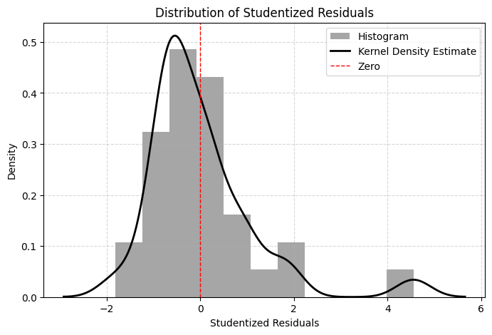

9.5 Least Absolute Deviations (LAD) Estimation¶

OLS minimizes the sum of squared residuals, which makes it sensitive to large outliers (since squaring magnifies large deviations). Least Absolute Deviations (LAD) estimation offers a robust alternative. LAD minimizes the sum of the absolute values of the residuals.

\min_{\beta_0, ..., \beta_k} \sum_{i=1}^n |y_i - \beta_0 - \beta_1 x_{i1} - ... - \beta_k x_{ik}|

(6)

LAD estimates are less sensitive to large outliers in the dependent variable $y$ .
LAD estimates the effect of $x$ on the conditional median of $y$ , whereas OLS estimates the effect on the conditional mean. These can differ if the error distribution is skewed.
LAD is a special case of quantile regression (estimating the median, i.e., the 0.5 quantile).

We compare OLS and LAD estimates for the R&D intensity model.

# Load data if needed
rdchem = wool.data("rdchem")

# --- OLS Regression ---
# Rescale sales for easier coefficient interpretation (sales in $billions)
reg_ols = smf.ols(formula="rdintens ~ I(sales/1000) + profmarg", data=rdchem)
results_ols = reg_ols.fit()

# --- OLS Estimation Results ---
table_ols = pd.DataFrame(
    {
        "b": round(results_ols.params, 4),
        "se": round(results_ols.bse, 4),
        "t": round(results_ols.tvalues, 4),
        "pval": round(results_ols.pvalues, 4),
    },
)
# OLS Estimates
table_ols

# --- LAD Regression (Quantile Regression at the Median) ---
# Use smf.quantreg and specify the quantile q=0.5 for LAD.
reg_lad = smf.quantreg(formula="rdintens ~ I(sales/1000) + profmarg", data=rdchem)
results_lad = reg_lad.fit(q=0.5)  # Fit for the median

# Display LAD results (statsmodels calculates SEs using appropriate methods for quantile regression)
# --- LAD (Median Regression) Estimation Results ---
table_lad = pd.DataFrame(
    {
        "b": round(results_lad.params, 4),  # LAD Coefficients
        "se": round(results_lad.bse, 4),  # LAD Standard Errors
        "t": round(results_lad.tvalues, 4),  # LAD t-statistics
        "pval": round(results_lad.pvalues, 4),  # LAD p-values
    },
)
# LAD Estimates
table_lad

# Interpretation (OLS vs LAD):
# - The coefficient on sales/1000 is 0.0534 (OLS) vs 0.0186 (LAD).
# - The coefficient on profit margin is 0.0446 (OLS) vs 0.1179 (LAD).
# - The intercept is also different.
# The differences suggest that the relationship might differ between the conditional mean (OLS)
# and the conditional median (LAD), possibly due to outliers or skewness in the conditional
# distribution of rdintens. The profit margin effect seems quite different across methods (LAD shows
# a larger coefficient and higher significance), while the sales effect is much smaller and insignificant
# in LAD. Since we identified potential outliers earlier, the LAD estimates might be considered more robust.

9.6 Using Proxy Variables for Unobserved Explanatory Variables¶

A common problem in empirical work is omitted variable bias (OVB): we want to include a variable in our regression that theoretically belongs there, but we cannot observe or measure it directly. A proxy variable is an observable variable that is related to the unobserved variable and can help reduce omitted variable bias.

9.6.1 The Proxy Variable Solution¶

Setup:

True model includes an unobserved variable $a^*$ :

y = \beta_0 + \beta_1 x_1 + \cdots + \beta_k x_k + \beta_{k+1} a^* + u

(7)

where:

$a^*$ is unobserved (e.g., ability, quality, managerial talent)
$u$ is the error term, uncorrelated with $(x_1, \ldots, x_k, a^*)$

Problem:

If we simply omit $a^*$ and regress $y$ on $(x_1, \ldots, x_k)$ , the OLS estimators will be biased if any $x_j$ is correlated with $a^*$ .

Proxy variable solution:

We observe a proxy $a$ that is related to $a^*$ :

a^* = \delta_0 + \delta_1 a + v

(8)

where $v$ is uncorrelated with $(a, x_1, \ldots, x_k, u)$ .

Key assumption: The proxy $a$ captures all the variation in $a^*$ that is correlated with the $x$ variables and $y$ .

Implementation:

Instead of the true model, we estimate:

y = \alpha_0 + \alpha_1 x_1 + \cdots + \alpha_k x_k + \alpha_{k+1} a + \text{error}

(9)

Result:

If the proxy variable assumptions hold, the OLS estimators of $\alpha_1, \ldots, \alpha_k$ from this regression are consistent for the true parameters $\beta_1, \ldots, \beta_k$ .

9.6.2 Properties of a Good Proxy Variable¶

A good proxy variable should:

Be correlated with the unobserved variable ( $\delta_1 \neq 0$ )
- If $a$ is uncorrelated with $a^*$ , it provides no information
Conditional on the proxy, the unobserved part is uncorrelated with explanatory variables
- Formally: $\text{Cov}(v, x_j) = 0$ for all $j$
- This means $a$ “soaks up” all the problematic correlation between $a^*$ and $x$
Be measured accurately (no measurement error in $a$ )

Examples of proxy variables:

Ability (unobserved): Use IQ score, test scores, or educational attainment as proxies
Firm quality (unobserved): Use past profitability, market share, or credit rating
Health status (partially observed): Use self-reported health, BMI, or smoking status
Neighborhood quality: Use median house prices, crime rates, or school test scores

9.6.3 Example: Returns to Education with Ability Proxy¶

Consider estimating the return to education on wages:

\log(\text{wage}) = \beta_0 + \beta_1 \text{educ} + \beta_2 \text{exper} + \beta_3 \text{ability} + u

(10)

Problem: Ability is unobserved, and likely correlated with education (more able people get more education).

Proxy solution: Use IQ score as a proxy for ability.

# Simulated example: Returns to education with ability proxy
np.random.seed(42)
n = 1000

# Generate unobserved ability
ability_star = np.random.normal(100, 15, n)

# Generate IQ as proxy for ability (with some noise)
# IQ = ability* + noise
iq = ability_star + np.random.normal(0, 10, n)

# Generate education (correlated with ability)
# More able people get more education
educ = 12 + 0.05 * ability_star + np.random.normal(0, 2, n)
educ = np.clip(educ, 8, 20)  # Cap between 8 and 20 years

# Generate experience (independent of ability for simplicity)
exper = np.random.uniform(0, 40, n)

# Generate log wages (depends on educ, exper, and ability)
log_wage = (
    1.5  # Intercept
    + 0.08 * educ  # True return to education
    + 0.02 * exper  # Experience effect
    + 0.005 * ability_star  # Ability effect
    + np.random.normal(0, 0.3, n)  # Error term
)

# Create DataFrame
wage_data = pd.DataFrame(
    {
        "log_wage": log_wage,
        "educ": educ,
        "exper": exper,
        "ability_star": ability_star,  # Unobserved in practice
        "iq": iq,  # Observed proxy
    },
)

print("Education-Ability correlation:", np.corrcoef(educ, ability_star)[0, 1].round(3))
print("IQ-Ability correlation:", np.corrcoef(iq, ability_star)[0, 1].round(3))

Education-Ability correlation: 0.365
IQ-Ability correlation: 0.82

Model 1: Naive regression (omitting ability)

# Model without ability (omitted variable bias)
model_naive = smf.ols(formula="log_wage ~ educ + exper", data=wage_data)
results_naive = model_naive.fit()

print("\nModel 1: Naive (Omitting Ability)")
print(f"Education coefficient: {results_naive.params['educ']:.4f}")
print(f"  (True value: 0.0800)")
print(f"  Bias: {results_naive.params['educ'] - 0.08:.4f}")


Model 1: Naive (Omitting Ability)
Education coefficient: 0.0970
  (True value: 0.0800)
  Bias: 0.0170

Model 2: Using IQ as proxy

# Model with IQ as proxy for ability
model_proxy = smf.ols(formula="log_wage ~ educ + exper + iq", data=wage_data)
results_proxy = model_proxy.fit()

print("\nModel 2: With IQ Proxy")
print(f"Education coefficient: {results_proxy.params['educ']:.4f}")
print(f"  (True value: 0.0800)")
print(f"  Bias: {results_proxy.params['educ'] - 0.08:.4f}")


Model 2: With IQ Proxy
Education coefficient: 0.0884
  (True value: 0.0800)
  Bias: 0.0084

Model 3: Oracle (using true ability - infeasible in practice)

# Model with true ability (infeasible in reality)
model_oracle = smf.ols(
    formula="log_wage ~ educ + exper + ability_star",
    data=wage_data,
)
results_oracle = model_oracle.fit()

print("\nModel 3: Oracle (True Ability - Infeasible)")
print(f"Education coefficient: {results_oracle.params['educ']:.4f}")
print(f"  (True value: 0.0800)")

# Comparison table
comparison_proxy = pd.DataFrame(
    {
        "Model": ["Naive (OVB)", "With IQ Proxy", "Oracle (True Ability)"],
        "Educ Coef": [
            results_naive.params["educ"],
            results_proxy.params["educ"],
            results_oracle.params["educ"],
        ],
        "Educ SE": [
            results_naive.bse["educ"],
            results_proxy.bse["educ"],
            results_oracle.bse["educ"],
        ],
        "Bias": [
            results_naive.params["educ"] - 0.08,
            results_proxy.params["educ"] - 0.08,
            results_oracle.params["educ"] - 0.08,
        ],
    },
)
print("\nComparison of Education Coefficient Estimates:")
comparison_proxy.round(4)

Interpretation:

The naive model overestimates the return to education due to omitted ability bias (able people earn more AND get more education)
Using IQ as a proxy substantially reduces the bias compared to the naive model
The proxy model gets closer to the oracle estimate (using true ability), though not perfectly
The quality of the proxy determines how much bias reduction we achieve

9.6.4 Limitations of Proxy Variables¶

Finding a good proxy is difficult
- Must satisfy strong assumptions (captures all relevant variation)
- Most proxies are imperfect
Proxy variables with measurement error
- If the proxy itself has measurement error, bias reduction is limited
Multiple unobservables
- If multiple unobserved variables matter, need multiple proxies
- Joint proxy assumptions become harder to satisfy
Alternative solutions may be better
- Instrumental variables (Chapter 15) can handle correlation without needing proxies
- Fixed effects (Chapter 14) for panel data can eliminate time-invariant unobservables
- Randomized experiments eliminate omitted variable bias entirely

When to use proxy variables:

When a theoretically important variable is unobserved
When you have a credible proxy (e.g., test scores for ability)
As a robustness check alongside other methods
When IV or fixed effects are not available

9.7 Models with Random Slopes¶

In standard regression, we assume coefficients are constant across all observations:

y_i = \beta_0 + \beta_1 x_{i1} + \cdots + \beta_k x_{ik} + u_i

(11)

But in many applications, the effect of $x$ on $y$ may vary across individuals, firms, or time periods. This leads to random coefficient models (also called random slope models or varying coefficient models).

9.7.1 Random Coefficient Specification¶

A simple random coefficient model:

y_i = \beta_{0i} + \beta_{1i} x_i + u_i

(12)

where $\beta_{0i}$ and $\beta_{1i}$ vary across observations.

Decomposition:

We can decompose the random coefficients into:

\beta_{0i} = \beta_0 + a_{0i}, \quad \beta_{1i} = \beta_1 + a_{1i}

(13)

where:

$\beta_0, \beta_1$ are the average coefficients
$a_{0i}, a_{1i}$ are individual-specific deviations from the average

Substituting:

y_i = (\beta_0 + a_{0i}) + (\beta_1 + a_{1i}) x_i + u_i

(14)

y_i = \beta_0 + \beta_1 x_i + \underbrace{(a_{0i} + a_{1i} x_i + u_i)}_{\text{composite error } v_i}

(15)

9.7.2 Implications for OLS¶

Key question: Can we estimate $\beta_0$ and $\beta_1$ (the average effects) using OLS?

Assumptions needed:

Independence: $E(a_{0i} | x_i) = 0$ and $E(a_{1i} | x_i) = 0$
- The individual deviations are uncorrelated with $x$
- This is the random coefficients assumption
Zero conditional mean: $E(u_i | x_i) = 0$ (standard assumption)

Under these assumptions:

E(y_i | x_i) = \beta_0 + \beta_1 x_i

(16)

So OLS is unbiased and consistent for $\beta_0$ and $\beta_1$ (the average coefficients).

However:

The composite error $v_i = a_{0i} + a_{1i} x_i + u_i$ is generally heteroskedastic:

\text{Var}(v_i | x_i) = \text{Var}(a_{0i}) + x_i^2 \text{Var}(a_{1i}) + 2x_i \text{Cov}(a_{0i}, a_{1i}) + \sigma_u^2

(17)

This variance depends on $x_i$ (specifically, quadratically through $x_i^2$ ).

Consequences:

OLS is still consistent for average effects $\beta_0, \beta_1$
Standard errors are incorrect - must use heteroskedasticity-robust SEs (Chapter 8)
OLS is not efficient - GLS or WLS could do better
Individual predictions $\hat{y}_i = \hat{\beta}_0 + \hat{\beta}_1 x_i$ predict the conditional mean, not individual $y_i$

9.7.3 Example: Returns to Education Varying by Ability¶

Suppose the return to education varies by unobserved ability:

\log(\text{wage}_i) = \beta_0 + (\beta_1 + a_i) \cdot \text{educ}_i + u_i

(18)

where $a_i$ is individual-specific deviation in the education return (correlated with ability).

# Simulate random coefficient model
np.random.seed(123)
n = 500

# Generate education
educ = np.random.uniform(8, 20, n)

# Generate random slope deviations (varying returns to education)
# Assume E(a_i | educ) = 0 (independence)
a_i = np.random.normal(0, 0.02, n)  # SD = 0.02

# Generate wages with random coefficients
# log(wage) = 1.0 + (0.10 + a_i)*educ + u
beta0_true = 1.0
beta1_avg = 0.10  # Average return to education
u = np.random.normal(0, 0.3, n)

log_wage_rc = beta0_true + (beta1_avg + a_i) * educ + u

rc_data = pd.DataFrame({"log_wage": log_wage_rc, "educ": educ})

# Estimate with OLS
model_rc = smf.ols(formula="log_wage ~ educ", data=rc_data)
results_rc_usual = model_rc.fit()
results_rc_robust = model_rc.fit(cov_type="HC3")

# Compare usual vs robust SEs
print("Random Coefficient Model: OLS Estimation")
print(f"Education coefficient: {results_rc_usual.params['educ']:.4f}")
print(f"  (True average: {beta1_avg:.4f})")
print(f"Standard error (usual): {results_rc_usual.bse['educ']:.4f}")
print(f"Standard error (robust): {results_rc_robust.bse['educ']:.4f}")
print(f"  Ratio (robust/usual): {results_rc_robust.bse['educ']/results_rc_usual.bse['educ']:.3f}")

# Demonstrate heteroskedasticity due to random slopes
# Variance of residuals should increase with educ^2
residuals = results_rc_usual.resid
rc_data["resid_sq"] = residuals**2
rc_data["educ_sq"] = educ**2

# Regress squared residuals on educ and educ^2 (heteroskedasticity test)
het_test = smf.ols(formula="resid_sq ~ educ + educ_sq", data=rc_data).fit()
print(f"\nHeteroskedasticity test (educ^2 coefficient): {het_test.params['educ_sq']:.4f}")
print(f"  p-value: {het_test.pvalues['educ_sq']:.4f}")
if het_test.pvalues["educ_sq"] < 0.05:
    print("  -> Significant heteroskedasticity (as expected with random slopes)")

Random Coefficient Model: OLS Estimation
Education coefficient: 0.1045
  (True average: 0.1000)
Standard error (usual): 0.0052
Standard error (robust): 0.0051
  Ratio (robust/usual): 0.988

Heteroskedasticity test (educ^2 coefficient): -0.0006
  p-value: 0.4571

Interpretation:

OLS estimates the average return to education consistently
Robust SEs are larger than usual SEs (accounting for heteroskedasticity)
Residual variance increases with $x^2$ (evidence of random slopes)
Always use robust standard errors when random coefficients are suspected

9.7.4 When Do Random Coefficients Matter?¶

Examples where coefficients likely vary:

Returns to education: Vary by ability, field, location
Price elasticity: Varies across consumers (income, preferences)
Treatment effects: Vary by individual characteristics (heterogeneous effects)
Production functions: Vary by firm technology or management
Regional policies: Same policy, different regional impacts

Practical implications:

Standard practice: Use robust SEs to account for potential random coefficients
Advanced models:
- Quantile regression (Section 9.5) estimates effects at different points of conditional distribution
- Interaction terms (Chapter 7) allow effects to vary with observables
- Panel data random effects (Chapter 14) model individual-specific coefficients
- Machine learning methods can estimate heterogeneous effects

Key takeaway:

Even if coefficients vary randomly across observations, OLS still consistently estimates the average effect as long as the coefficient variation is independent of $x$ . However, heteroskedasticity-robust inference is essential since the error variance is non-constant.

Chapter Summary¶

This chapter addressed critical specification and data issues that arise frequently in empirical econometric work. While earlier chapters assumed the model was correctly specified with clean data, real-world analysis requires careful attention to functional form, measurement quality, missing observations, outliers, and alternative estimation methods. Understanding these issues is essential for producing credible and robust research.

9.1 Key Concepts¶

Functional Form Misspecification

Linear-in-variables vs linear-in-parameters: OLS requires linearity in parameters but allows flexible functional forms
Logarithms for percentage effects and elasticities
Polynomials (quadratic, cubic) for non-linear relationships
Interactions between variables for effect modification
RESET test detects functional form misspecification using powers of fitted values
Davidson-MacKinnon test (J-test) compares non-nested models

Measurement Error

Measurement error in $y$ (dependent variable): Absorbed into error term, increases variance but doesn’t bias coefficients
Measurement error in $x$ (explanatory variable): Causes attenuation bias toward zero (underestimate true effect)
Classical measurement error: $x^* = x + e$ where $e$ is uncorrelated with true $x^*$ and other variables
Proxy variables: Use observable correlated variable to reduce omitted variable bias

Missing Data

Missing completely at random (MCAR): Missingness independent of all variables - no bias but loses efficiency
Missing at random (MAR): Missingness depends on observables - bias if not controlled
Missing not at random (MNAR): Missingness depends on unobservables - leads to sample selection bias

Outliers and Influential Observations

Outliers: Observations far from the regression line (large residuals)
Leverage: Observations with extreme $x$ values that can heavily influence estimates
Influential points: Combine high leverage with unusual $y$ values
Diagnostic tools: Residual plots, leverage statistics, Cook’s distance, DFBETAS

Robust Estimation

Least Absolute Deviations (LAD): Minimizes absolute deviations, more robust to outliers
Estimates conditional median instead of conditional mean
Less efficient than OLS when errors are normal
More robust when errors are heavy-tailed or outliers present

9.2 Python Implementation Patterns¶

Functional Form Testing

# RESET test
from statsmodels.stats.diagnostic import linear_reset

reset_stat, reset_pval, _ = linear_reset(results, power=2)
# Reject H0 (linear) if p-value < 0.05

# Davidson-MacKinnon J-test
fitted_model2 = results_model2.fittedvalues
data['y_hat_2'] = fitted_model2
augmented_model1 = smf.ols('y ~ x1 + x2 + y_hat_2', data=data).fit()
# Check significance of y_hat_2

Measurement Error Simulation

# Generate measurement error
x_star = true_x
x_measured = x_star + np.random.normal(0, sigma_e, n)

# Attenuation factor
attenuation = sigma_x**2 / (sigma_x**2 + sigma_e**2)
# E(beta_hat) = attenuation * beta_true

Missing Data Handling

# Check missingness patterns
data.isnull().sum()
data[data['variable'].isnull()].describe()

# Listwise deletion (complete case analysis)
data_complete = data.dropna()

# Create missingness indicator
data['missing_x'] = data['x'].isnull().astype(int)

Outlier Detection

# Standardized residuals
from scipy import stats
standardized = results.resid / np.std(results.resid)
outliers = np.abs(standardized) > 3

# Leverage
from statsmodels.stats.outliers_influence import OLSInfluence
influence = OLSInfluence(results)
leverage = influence.hat_matrix_diag
high_leverage = leverage > 2 * k / n  # Rule of thumb

# Cook's distance
cooks_d = influence.cooks_distance[0]
influential = cooks_d > 4 / n

LAD Estimation

# Quantile regression at median (LAD)
import statsmodels.formula.api as smf
model_lad = smf.quantreg('y ~ x1 + x2', data=data)
results_lad = model_lad.fit(q=0.5)  # q=0.5 for median

Proxy Variables

# Include proxy in regression to reduce OVB
model_proxy = smf.ols('y ~ x + proxy_for_omitted', data=data).fit()
# Compare to naive model without proxy

9.3 Common Pitfalls and Best Practices¶

Functional Form

DON’T: Use linear specification for all relationships without investigation DO: Plot $y$ vs $x$ to visualize relationship before modeling DO: Use RESET or graphical diagnostics to test specification DO: Consider economic theory when choosing functional forms

Measurement Error

DON’T: Ignore that administrative or survey data may have measurement error DON’T: Use variables with large measurement error as key explanatory variables DO: Understand which variables are measured accurately DO: Report results both with and without noisy variables DO: Consider instrumental variables (Chapter 15) if measurement error is severe

Missing Data

DON’T: Delete missing observations without investigating the pattern DON’T: Assume MCAR when missingness might depend on outcomes DO: Document how many observations are lost and why DO: Compare characteristics of complete vs incomplete cases DO: Test whether missingness predicts outcomes DO: Use selection correction methods (Chapter 17) if MNAR is likely

Outliers

DON’T: Automatically delete outliers without justification DON’T: Ignore outliers that contradict your hypothesis DO: Identify outliers using multiple diagnostics (residuals + leverage) DO: Investigate whether outliers are data errors or genuine extreme values DO: Report results with and without outliers DO: Use robust methods (LAD, robust SEs) as sensitivity checks

General Best Practices

Exploratory data analysis: Always examine distributions, relationships, and data quality before modeling
Diagnostic plots: Use residual plots, Q-Q plots, leverage plots routinely
Robustness checks: Estimate models with different specifications, subsamples, methods
Transparency: Report all specification searches and sensitivity analyses
Domain knowledge: Use economic theory and institutional knowledge to guide specification

9.4 Decision Framework¶

Choosing Functional Form:

Theory: What functional form does economic theory suggest? (e.g., Cobb-Douglas → logs)
Data: Plot relationships - are they linear, curved, or non-monotonic?
Testing: Run RESET test - does it reject linear specification?
Interpretation: Will logs or polynomials aid interpretation? (elasticities, turning points)
Comparison: Use AIC/BIC or cross-validation to compare nested/non-nested models

Handling Measurement Error:

Situation	Best Approach
Error in $y$ only	Standard OLS (unbiased)
Small error in $x$	OLS + robust SEs + acknowledge limitation
Large error in $x$	Find better data or use IV (Chapter 15)
Error in multiple variables	IV or errors-in-variables models

Handling Missing Data:

Missingness Type	Strategy
MCAR (rare)	Complete case analysis acceptable (inefficient)
MAR	Include variables predicting missingness as controls
MNAR	Selection models (Chapter 17) or bound analysis
Large missingness	Report with/without imputation; document assumptions

Handling Outliers:

Decision Tree:
1. Are outliers data errors?
   -> YES: Correct or delete (document correction)
   -> NO: Proceed to step 2

2. Are they from the target population?
   -> NO: Consider separate analysis or exclusion (justify)
   -> YES: Proceed to step 3

3. Do they change substantive conclusions?
   -> NO: Report main results, note robustness
   -> YES: Proceed to step 4

4. Reporting strategy:
   - Main results with outliers (full sample)
   - Robustness with LAD or winsorization
   - Sensitivity analysis excluding outliers
   - Explain which you prefer and why

9.5 Connections to Other Chapters¶

To Chapter 6 (Further Issues in MRA):

Builds on functional form discussion (logs, interactions from Ch6)
Extends scaling and measurement concerns
Connects proxy variables to omitted variable bias (Ch6.3)

To Chapter 8 (Heteroskedasticity):

Random coefficients (Section 9.7) naturally create heteroskedasticity
Robust SEs essential when coefficient variation suspected
LAD as alternative to WLS for dealing with non-constant variance

To Chapter 13-14 (Panel Data):

Fixed effects eliminate time-invariant measurement error
Panel data allows differencing out individual-specific unobservables (proxy alternative)
Random effects are special case of random coefficients

To Chapter 15 (Instrumental Variables):

IV solution to measurement error in $x$ more general than proxies
Both address endogeneity but with different assumptions
IV requires excluded instruments; proxies require inclusion restrictions

To Chapter 17 (Limited Dependent Variables):

Sample selection is special case of MNAR missing data
Heckman correction formally models selection process
Tobit model handles censored data (special missingness case)

9.6 Mathematical Summary¶

Functional Form:

True model: $y = g(x_1, \ldots, x_k, u)$

Approximation: $y \approx \beta_0 + \beta_1 h_1(x) + \cdots + \beta_p h_p(x) + \text{error}$

where $h_j(x)$ are transformations (logs, polynomials, interactions).

RESET statistic:

F = \frac{(\text{SSR}_{\text{restricted}} - \text{SSR}_{\text{unrestricted}})/q}{\text{SSR}_{\text{unrestricted}}/(n - k_{\text{unrestricted}})}

(19)

Measurement error in $x$ :

True model: $y = \beta_0 + \beta_1 x^* + u$

Observed: $x = x^* + e$ where $\text{Cov}(x^*, e) = 0$

Attenuation bias:

\text{plim} \, \hat{\beta}_1 = \beta_1 \cdot \frac{\text{Var}(x^*)}{\text{Var}(x^*) + \text{Var}(e)} = \beta_1 \cdot \lambda

(20)

where $0 < \lambda < 1$ (attenuation factor).

Proxy variables:

Unobserved: $y = \beta_0 + \beta_1 x + \beta_2 a^* + u$

Proxy relation: $a^* = \delta_0 + \delta_1 a + v$ where $\text{Cov}(v, x) = 0$

Estimated model: $y = \alpha_0 + \alpha_1 x + \alpha_2 a + \text{error}$

Under proxy assumptions: $\hat{\alpha}_1 \xrightarrow{p} \beta_1$ (consistent for effect of $x$ )

Random coefficients:

y_i = \beta_{0i} + \beta_{1i} x_i + u_i = (\beta_0 + a_{0i}) + (\beta_1 + a_{1i}) x_i + u_i

(21)

Composite error: $v_i = a_{0i} + a_{1i} x_i + u_i$

Heteroskedasticity:

\text{Var}(v_i | x_i) = \sigma_{a_0}^2 + x_i^2 \sigma_{a_1}^2 + 2x_i \sigma_{a_0 a_1} + \sigma_u^2

(22)

LAD estimator:

\hat{\beta}_{\text{LAD}} = \arg\min_{\beta} \sum_{i=1}^n |y_i - x_i' \beta|

(23)

Estimates: $\text{Median}(y | x)$ instead of $E(y | x)$

9.7 Learning Objectives Recap¶

This chapter covered all 11 learning objectives:

9.1 - Explain why choosing the wrong functional form can bias coefficient estimates and describe methods to test for and correct functional form misspecification

9.2 - Understand the consequences of using proxy variables for unobserved explanatory variables and the assumptions required for valid inference

9.3 - Analyze the implications of models with random slopes (random coefficients) and explain why heteroskedasticity-robust standard errors are necessary

9.4 - Apply the RESET test to detect functional form misspecification and interpret results

9.5 - Conduct Davidson-MacKinnon J-tests to compare non-nested model specifications

9.6 - Demonstrate how measurement error in the dependent variable affects OLS estimates differently than measurement error in explanatory variables

9.7 - Explain the attenuation bias that results from classical measurement error in explanatory variables and calculate the bias analytically

9.8 - Distinguish between missing completely at random (MCAR), missing at random (MAR), and missing not at random (MNAR), and select appropriate methods for each

9.9 - Identify outliers and influential observations using residual analysis, leverage statistics, and Cook’s distance

9.10 - Implement Least Absolute Deviations (LAD) estimation as a robust alternative to OLS when outliers are present

9.11 - Conduct comprehensive specification and data quality diagnostics for empirical projects, including functional form tests, outlier detection, and missing data analysis

9.8 Further Reading and Extensions¶

Advanced topics not covered:

Imputation methods: Multiple imputation, EM algorithm for handling missing data
Robust regression: M-estimators, Huber regression, bounded influence estimators
Non-parametric regression: Kernel regression, local polynomial regression, splines
Model averaging: Combining predictions from multiple specifications
Diagnostic testing: Leverage plots, partial regression plots, added variable plots

Recommended resources:

Wooldridge (2020), Chapters 9 and 17 for theoretical foundations
Cameron & Trivedi (2005), “Microeconometrics” for advanced treatment of missing data and outliers
Angrist & Pischke (2009), “Mostly Harmless Econometrics” for practical specification advice
Fox (2016), “Applied Regression Analysis and GLMs in R” for extensive diagnostic methods
Heiss (2020), “Using Python for Introductory Econometrics” for Python implementations

This chapter equipped you with essential tools for data cleaning, model specification, and robust analysis. Applying these methods systematically will improve the credibility and replicability of empirical work in economics and related fields.

merino

Chapter 8: Heteroskedasticity

merino

Chapter 10: Basic Regression Analysis with Time Series Data

Chapter 9: Specification and Data Issues

9.1 Functional Form Misspecification¶

9.1.1 The RESET Test¶

9.1.2 Example: Housing Price Equation¶

Non-nested Tests (Davidson-MacKinnon)¶

9.2 Measurement Error¶

Measurement Error in the Dependent Variable (yyy)¶

Measurement Error in an Independent Variable (xxx)¶

Simulation: Measurement Error in yyy¶

Simulation: Measurement Error in xxx¶

9.3 Missing Data and Nonrandom Samples¶

9.4 Outlying Observations¶

9.5 Least Absolute Deviations (LAD) Estimation¶

9.6 Using Proxy Variables for Unobserved Explanatory Variables¶

9.6.1 The Proxy Variable Solution¶

9.6.2 Properties of a Good Proxy Variable¶

9.6.3 Example: Returns to Education with Ability Proxy¶

9.6.4 Limitations of Proxy Variables¶

9.7 Models with Random Slopes¶

9.7.1 Random Coefficient Specification¶

9.7.2 Implications for OLS¶

9.7.3 Example: Returns to Education Varying by Ability¶

9.7.4 When Do Random Coefficients Matter?¶

Chapter Summary¶

9.1 Key Concepts¶

9.2 Python Implementation Patterns¶

9.3 Common Pitfalls and Best Practices¶

9.4 Decision Framework¶

9.5 Connections to Other Chapters¶

9.6 Mathematical Summary¶

9.7 Learning Objectives Recap¶

9.8 Further Reading and Extensions¶

Measurement Error in the Dependent Variable ( $y$ )¶

Measurement Error in an Independent Variable ( $x$ )¶

Simulation: Measurement Error in $y$ ¶

Simulation: Measurement Error in $x$ ¶